Cubic Equations of State (thermo.eos)

This module contains implementations of most cubic equations of state for pure components. This includes Peng-Robinson, SRK, Van der Waals, PRSV, TWU and many other variants.

For reporting bugs, adding feature requests, or submitting pull requests, please use the GitHub issue tracker.

Base Class

class thermo.eos.GCEOS

Bases: object

Class for solving a generic Pressure-explicit three-parameter cubic equation of state. Does not implement any parameters itself; must be subclassed by an equation of state class which uses it. Works for mixtures or pure species for all properties except fugacity. All properties are derived with the CAS SymPy, not relying on any derivations previously published.

$$P=\frac{RT}{V-b}-\frac{a\alpha(T)}{V^2 + \delta V + \epsilon}$$

The main methods (in order they are called) are GCEOS.solve, GCEOS.set_from_PT, GCEOS.volume_solutions, and GCEOS.set_properties_from_solution.

GCEOS.solve calls GCEOS.check_sufficient_inputs, which checks if two of T, P, and V were set. It then solves for the remaining variable. If T is missing, method GCEOS.solve_T is used; it is parameter specific, and so must be implemented in each specific EOS. If P is missing, it is directly calculated. If V is missing, it is calculated with the method GCEOS.volume_solutions. At this point, either three possible volumes or one user specified volume are known. The value of a_alpha, and its first and second temperature derivative are calculated with the EOS-specific method GCEOS.a_alpha_and_derivatives.

If V is not provided, GCEOS.volume_solutions calculates the three possible molar volumes which are solutions to the EOS; in the single-phase region, only one solution is real and correct. In the two-phase region, all volumes are real, but only the largest and smallest solution are physically meaningful, with the largest being that of the gas and the smallest that of the liquid.

GCEOS.set_from_PT is called to sort out the possible molar volumes. For the case of a user-specified V, the possibility of there existing another solution is ignored for speed. If there is only one real volume, the method GCEOS.set_properties_from_solution is called with it. If there are two real volumes, GCEOS.set_properties_from_solution is called once with each volume. The phase is returned by GCEOS.set_properties_from_solution, and the volumes is set to either GCEOS.V_l or GCEOS.V_g as appropriate.

GCEOS.set_properties_from_solution is a large function which calculates all relevant partial derivatives and properties of the EOS. 17 derivatives and excess enthalpy and entropy are calculated first. Finally, it sets all these properties as attibutes for either the liquid or gas phase with the convention of adding on _l or _g to the variable names, respectively.

Attributes

Tfloat

Temperature of cubic EOS state, [K]

Pfloat

Pressure of cubic EOS state, [Pa]

afloat

a parameter of cubic EOS; formulas vary with the EOS, [Pa*m^6/mol^2]

bfloat

b parameter of cubic EOS; formulas vary with the EOS, [m^3/mol]

deltafloat

Coefficient calculated by EOS-specific method, [m^3/mol]

epsilonfloat

Coefficient calculated by EOS-specific method, [m^6/mol^2]

a_alphafloat

Coefficient calculated by EOS-specific method, [J^2/mol^2/Pa]

da_alpha_dTfloat

Temperature derivative of $a \alpha$ calculated by EOS-specific method, [J^2/mol^2/Pa/K]

d2a_alpha_dT2float

Second temperature derivative of $a \alpha$ calculated by EOS-specific method, [J^2/mol^2/Pa/K**2]

Zcfloat

Critical compressibility of cubic EOS state, [-]

phasestr

One of ‘l’, ‘g’, or ‘l/g’ to represent whether or not there is a liquid-like solution, vapor-like solution, or both available, [-]

raw_volumeslist[(float, complex), 3]

Calculated molar volumes from the volume solver; depending on the state and selected volume solver, imaginary volumes may be represented by 0 or -1j to save the time of actually calculating them, [m^3/mol]

V_lfloat

Liquid phase molar volume, [m^3/mol]

V_gfloat

Vapor phase molar volume, [m^3/mol]

Vfloat or None

Molar volume specified as input; otherwise None, [m^3/mol]

Z_lfloat

Liquid phase compressibility, [-]

Z_gfloat

Vapor phase compressibility, [-]

PIP_lfloat

Liquid phase phase identification parameter, [-]

PIP_gfloat

Vapor phase phase identification parameter, [-]

dP_dT_lfloat

Liquid phase temperature derivative of pressure at constant volume, [Pa/K].

$$\left(\frac{\partial P}{\partial T}\right)_V = \frac{R}{V - b} - \frac{a \frac{d \alpha{\left (T \right )}}{d T}}{V^{2} + V \delta + \epsilon}$$

dP_dT_gfloat

Vapor phase temperature derivative of pressure at constant volume, [Pa/K].

$$\left(\frac{\partial P}{\partial T}\right)_V = \frac{R}{V - b} - \frac{a \frac{d \alpha{\left (T \right )}}{d T}}{V^{2} + V \delta + \epsilon}$$

dP_dV_lfloat

Liquid phase volume derivative of pressure at constant temperature, [Pa*mol/m^3].

$$\left(\frac{\partial P}{\partial V}\right)_T = - \frac{R T}{\left( V - b\right)^{2}} - \frac{a \left(- 2 V - \delta\right) \alpha{ \left (T \right )}}{\left(V^{2} + V \delta + \epsilon\right)^{2}}$$

dP_dV_gfloat

Gas phase volume derivative of pressure at constant temperature, [Pa*mol/m^3].

$$\left(\frac{\partial P}{\partial V}\right)_T = - \frac{R T}{\left( V - b\right)^{2}} - \frac{a \left(- 2 V - \delta\right) \alpha{ \left (T \right )}}{\left(V^{2} + V \delta + \epsilon\right)^{2}}$$

dV_dT_lfloat

Liquid phase temperature derivative of volume at constant pressure, [m^3/(mol*K)].

$$\left(\frac{\partial V}{\partial T}\right)_P =-\frac{ \left(\frac{\partial P}{\partial T}\right)_V}{ \left(\frac{\partial P}{\partial V}\right)_T}$$

dV_dT_gfloat

Gas phase temperature derivative of volume at constant pressure, [m^3/(mol*K)].

$$\left(\frac{\partial V}{\partial T}\right)_P =-\frac{ \left(\frac{\partial P}{\partial T}\right)_V}{ \left(\frac{\partial P}{\partial V}\right)_T}$$

dV_dP_lfloat

Liquid phase pressure derivative of volume at constant temperature, [m^3/(mol*Pa)].

$$\left(\frac{\partial V}{\partial P}\right)_T =-\frac{ \left(\frac{\partial V}{\partial T}\right)_P}{ \left(\frac{\partial P}{\partial T}\right)_V}$$

dV_dP_gfloat

Gas phase pressure derivative of volume at constant temperature, [m^3/(mol*Pa)].

$$\left(\frac{\partial V}{\partial P}\right)_T =-\frac{ \left(\frac{\partial V}{\partial T}\right)_P}{ \left(\frac{\partial P}{\partial T}\right)_V}$$

dT_dV_lfloat

Liquid phase volume derivative of temperature at constant pressure, [K*mol/m^3].

$$\left(\frac{\partial T}{\partial V}\right)_P = \frac{1} {\left(\frac{\partial V}{\partial T}\right)_P}$$

dT_dV_gfloat

Gas phase volume derivative of temperature at constant pressure, [K*mol/m^3]. See GCEOS.set_properties_from_solution for the formula.

dT_dP_lfloat

Liquid phase pressure derivative of temperature at constant volume, [K/Pa].

$$\left(\frac{\partial T}{\partial P}\right)_V = \frac{1} {\left(\frac{\partial P}{\partial T}\right)_V}$$

dT_dP_gfloat

Gas phase pressure derivative of temperature at constant volume, [K/Pa].

$$\left(\frac{\partial T}{\partial P}\right)_V = \frac{1} {\left(\frac{\partial P}{\partial T}\right)_V}$$

d2P_dT2_lfloat

Liquid phase second derivative of pressure with respect to temperature at constant volume, [Pa/K^2].

$$\left(\frac{\partial^2 P}{\partial T^2}\right)_V = - \frac{a \frac{d^{2} \alpha{\left (T \right )}}{d T^{2}}}{V^{2} + V \delta + \epsilon}$$

d2P_dT2_gfloat

Gas phase second derivative of pressure with respect to temperature at constant volume, [Pa/K^2].

$$\left(\frac{\partial^2 P}{\partial T^2}\right)_V = - \frac{a \frac{d^{2} \alpha{\left (T \right )}}{d T^{2}}}{V^{2} + V \delta + \epsilon}$$

d2P_dV2_lfloat

Liquid phase second derivative of pressure with respect to volume at constant temperature, [Pa*mol^2/m^6].

$$\left(\frac{\partial^2 P}{\partial V^2}\right)_T = 2 \left(\frac{ R T}{\left(V - b\right)^{3}} - \frac{a \left(2 V + \delta\right)^{ 2} \alpha{\left (T \right )}}{\left(V^{2} + V \delta + \epsilon \right)^{3}} + \frac{a \alpha{\left (T \right )}}{\left(V^{2} + V \delta + \epsilon\right)^{2}}\right)$$

d2P_dTdV_lfloat

Liquid phase second derivative of pressure with respect to volume and then temperature, [Pa*mol/(K*m^3)].

$$\left(\frac{\partial^2 P}{\partial T \partial V}\right) = - \frac{ R}{\left(V - b\right)^{2}} + \frac{a \left(2 V + \delta\right) \frac{d \alpha{\left (T \right )}}{d T}}{\left(V^{2} + V \delta + \epsilon\right)^{2}}$$

d2P_dTdV_gfloat

Gas phase second derivative of pressure with respect to volume and then temperature, [Pa*mol/(K*m^3)].

$$\left(\frac{\partial^2 P}{\partial T \partial V}\right) = - \frac{ R}{\left(V - b\right)^{2}} + \frac{a \left(2 V + \delta\right) \frac{d \alpha{\left (T \right )}}{d T}}{\left(V^{2} + V \delta + \epsilon\right)^{2}}$$

H_dep_lfloat

Liquid phase departure enthalpy, [J/mol]. See GCEOS.set_properties_from_solution for the formula.

H_dep_gfloat

Gas phase departure enthalpy, [J/mol]. See GCEOS.set_properties_from_solution for the formula.

S_dep_lfloat

Liquid phase departure entropy, [J/(mol*K)]. See GCEOS.set_properties_from_solution for the formula.

S_dep_gfloat

Gas phase departure entropy, [J/(mol*K)]. See GCEOS.set_properties_from_solution for the formula.

G_dep_lfloat

Liquid phase departure Gibbs energy, [J/mol].

$$G_{dep} = H_{dep} - T S_{dep}$$

G_dep_gfloat

Gas phase departure Gibbs energy, [J/mol].

$$G_{dep} = H_{dep} - T S_{dep}$$

Cp_dep_lfloat

Liquid phase departure heat capacity, [J/(mol*K)]

$$C_{p, dep} = (C_p-C_v)_{\text{from EOS}} + C_{v, dep} - R$$

Cp_dep_gfloat

Gas phase departure heat capacity, [J/(mol*K)]

$$C_{p, dep} = (C_p-C_v)_{\text{from EOS}} + C_{v, dep} - R$$

Cv_dep_lfloat

Liquid phase departure constant volume heat capacity, [J/(mol*K)]. See GCEOS.set_properties_from_solution for the formula.

Cv_dep_gfloat

Gas phase departure constant volume heat capacity, [J/(mol*K)]. See GCEOS.set_properties_from_solution for the formula.

c1float

Full value of the constant in the a parameter, set in some EOSs, [-]

c2float

Full value of the constant in the b parameter, set in some EOSs, [-]

A_dep_g

Departure molar Helmholtz energy from ideal gas behavior for the gas phase, [J/mol].

A_dep_l

Departure molar Helmholtz energy from ideal gas behavior for the liquid phase, [J/mol].

beta_g

Isobaric (constant-pressure) expansion coefficient for the gas phase, [1/K].

beta_l

Isobaric (constant-pressure) expansion coefficient for the liquid phase, [1/K].

Cp_minus_Cv_g

Cp - Cv for the gas phase, [J/mol/K].

Cp_minus_Cv_l

Cp - Cv for the liquid phase, [J/mol/K].

d2a_alpha_dTdP_g_V

Derivative of the temperature derivative of a_alpha with respect to pressure at constant volume (varying T) for the gas phase, [J^2/mol^2/Pa^2/K].

d2a_alpha_dTdP_l_V

Derivative of the temperature derivative of a_alpha with respect to pressure at constant volume (varying T) for the liquid phase, [J^2/mol^2/Pa^2/K].

d2H_dep_dT2_g

Second temperature derivative of departure enthalpy with respect to temperature for the gas phase, [(J/mol)/K^2].

d2H_dep_dT2_g_P

Second temperature derivative of departure enthalpy with respect to temperature for the gas phase, [(J/mol)/K^2].

d2H_dep_dT2_g_V

Second temperature derivative of departure enthalpy with respect to temperature at constant volume for the gas phase, [(J/mol)/K^2].

d2H_dep_dT2_l

Second temperature derivative of departure enthalpy with respect to temperature for the liquid phase, [(J/mol)/K^2].

d2H_dep_dT2_l_P

Second temperature derivative of departure enthalpy with respect to temperature for the liquid phase, [(J/mol)/K^2].

d2H_dep_dT2_l_V

Second temperature derivative of departure enthalpy with respect to temperature at constant volume for the liquid phase, [(J/mol)/K^2].

d2H_dep_dTdP_g

Temperature and pressure derivative of departure enthalpy at constant pressure then temperature for the gas phase, [(J/mol)/K/Pa].

d2H_dep_dTdP_l

Temperature and pressure derivative of departure enthalpy at constant pressure then temperature for the liquid phase, [(J/mol)/K/Pa].

d2P_drho2_g

Second derivative of pressure with respect to molar density for the gas phase, [Pa/(mol/m^3)^2].

d2P_drho2_l

Second derivative of pressure with respect to molar density for the liquid phase, [Pa/(mol/m^3)^2].

d2P_dT2_PV_g

Second derivative of pressure with respect to temperature twice, but with pressure held constant the first time and volume held constant the second time for the gas phase, [Pa/K^2].

d2P_dT2_PV_l

Second derivative of pressure with respect to temperature twice, but with pressure held constant the first time and volume held constant the second time for the liquid phase, [Pa/K^2].

d2P_dTdP_g

Second derivative of pressure with respect to temperature and, then pressure; and with volume held constant at first, then temperature, for the gas phase, [1/K].

d2P_dTdP_l

Second derivative of pressure with respect to temperature and, then pressure; and with volume held constant at first, then temperature, for the liquid phase, [1/K].

d2P_dTdrho_g

Derivative of pressure with respect to molar density, and temperature for the gas phase, [Pa/(K*mol/m^3)].

d2P_dTdrho_l

Derivative of pressure with respect to molar density, and temperature for the liquid phase, [Pa/(K*mol/m^3)].

d2P_dVdP_g

Second derivative of pressure with respect to molar volume and then pressure for the gas phase, [mol/m^3].

d2P_dVdP_l

Second derivative of pressure with respect to molar volume and then pressure for the liquid phase, [mol/m^3].

d2P_dVdT_g

Alias of GCEOS.d2P_dTdV_g

d2P_dVdT_l

Alias of GCEOS.d2P_dTdV_l

d2P_dVdT_TP_g

Second derivative of pressure with respect to molar volume and then temperature at constant temperature then pressure for the gas phase, [Pa*mol/m^3/K].

d2P_dVdT_TP_l

Second derivative of pressure with respect to molar volume and then temperature at constant temperature then pressure for the liquid phase, [Pa*mol/m^3/K].

d2rho_dP2_g

Second derivative of molar density with respect to pressure for the gas phase, [(mol/m^3)/Pa^2].

d2rho_dP2_l

Second derivative of molar density with respect to pressure for the liquid phase, [(mol/m^3)/Pa^2].

d2rho_dPdT_g

Second derivative of molar density with respect to pressure and temperature for the gas phase, [(mol/m^3)/(K*Pa)].

d2rho_dPdT_l

Second derivative of molar density with respect to pressure and temperature for the liquid phase, [(mol/m^3)/(K*Pa)].

d2rho_dT2_g

Second derivative of molar density with respect to temperature for the gas phase, [(mol/m^3)/K^2].

d2rho_dT2_l

Second derivative of molar density with respect to temperature for the liquid phase, [(mol/m^3)/K^2].

d2S_dep_dT2_g

Second temperature derivative of departure entropy with respect to temperature for the gas phase, [(J/mol)/K^3].

d2S_dep_dT2_g_V

Second temperature derivative of departure entropy with respect to temperature at constant volume for the gas phase, [(J/mol)/K^3].

d2S_dep_dT2_l

Second temperature derivative of departure entropy with respect to temperature for the liquid phase, [(J/mol)/K^3].

d2S_dep_dT2_l_V

Second temperature derivative of departure entropy with respect to temperature at constant volume for the liquid phase, [(J/mol)/K^3].

d2S_dep_dTdP_g

Temperature and pressure derivative of departure entropy at constant pressure then temperature for the gas phase, [(J/mol)/K^2/Pa].

d2S_dep_dTdP_l

Temperature and pressure derivative of departure entropy at constant pressure then temperature for the liquid phase, [(J/mol)/K^2/Pa].

d2T_dP2_g

Second partial derivative of temperature with respect to pressure (constant volume) for the gas phase, [K/Pa^2].

d2T_dP2_l

Second partial derivative of temperature with respect to pressure (constant temperature) for the liquid phase, [K/Pa^2].

d2T_dPdrho_g

Derivative of temperature with respect to molar density, and pressure for the gas phase, [K/(Pa*mol/m^3)].

d2T_dPdrho_l

Derivative of temperature with respect to molar density, and pressure for the liquid phase, [K/(Pa*mol/m^3)].

d2T_dPdV_g

Second partial derivative of temperature with respect to pressure (constant volume) and then volume (constant pressure) for the gas phase, [K*mol/(Pa*m^3)].

d2T_dPdV_l

Second partial derivative of temperature with respect to pressure (constant volume) and then volume (constant pressure) for the liquid phase, [K*mol/(Pa*m^3)].

d2T_drho2_g

Second derivative of temperature with respect to molar density for the gas phase, [K/(mol/m^3)^2].

d2T_drho2_l

Second derivative of temperature with respect to molar density for the liquid phase, [K/(mol/m^3)^2].

d2T_dV2_g

Second partial derivative of temperature with respect to volume (constant pressure) for the gas phase, [K*mol^2/m^6].

d2T_dV2_l

Second partial derivative of temperature with respect to volume (constant pressure) for the liquid phase, [K*mol^2/m^6].

d2T_dVdP_g

Second partial derivative of temperature with respect to pressure (constant volume) and then volume (constant pressure) for the gas phase, [K*mol/(Pa*m^3)].

d2T_dVdP_l

Second partial derivative of temperature with respect to pressure (constant volume) and then volume (constant pressure) for the liquid phase, [K*mol/(Pa*m^3)].

d2V_dP2_g

Second partial derivative of volume with respect to pressure (constant temperature) for the gas phase, [m^3/(Pa^2*mol)].

d2V_dP2_l

Second partial derivative of volume with respect to pressure (constant temperature) for the liquid phase, [m^3/(Pa^2*mol)].

d2V_dPdT_g

Second partial derivative of volume with respect to pressure (constant temperature) and then presssure (constant temperature) for the gas phase, [m^3/(K*Pa*mol)].

d2V_dPdT_l

Second partial derivative of volume with respect to pressure (constant temperature) and then presssure (constant temperature) for the liquid phase, [m^3/(K*Pa*mol)].

d2V_dT2_g

Second partial derivative of volume with respect to temperature (constant pressure) for the gas phase, [m^3/(mol*K^2)].

d2V_dT2_l

Second partial derivative of volume with respect to temperature (constant pressure) for the liquid phase, [m^3/(mol*K^2)].

d2V_dTdP_g

Second partial derivative of volume with respect to pressure (constant temperature) and then presssure (constant temperature) for the gas phase, [m^3/(K*Pa*mol)].

d2V_dTdP_l

Second partial derivative of volume with respect to pressure (constant temperature) and then presssure (constant temperature) for the liquid phase, [m^3/(K*Pa*mol)].

d3a_alpha_dT3

Method to calculate the third temperature derivative of $a \alpha$, [J^2/mol^2/Pa/K^3].

da_alpha_dP_g_V

Derivative of the a_alpha with respect to pressure at constant volume (varying T) for the gas phase, [J^2/mol^2/Pa^2].

da_alpha_dP_l_V

Derivative of the a_alpha with respect to pressure at constant volume (varying T) for the liquid phase, [J^2/mol^2/Pa^2].

dbeta_dP_g

Derivative of isobaric expansion coefficient with respect to pressure for the gas phase, [1/(Pa*K)].

dbeta_dP_l

Derivative of isobaric expansion coefficient with respect to pressure for the liquid phase, [1/(Pa*K)].

dbeta_dT_g

Derivative of isobaric expansion coefficient with respect to temperature for the gas phase, [1/K^2].

dbeta_dT_l

Derivative of isobaric expansion coefficient with respect to temperature for the liquid phase, [1/K^2].

dfugacity_dP_g

Derivative of fugacity with respect to pressure for the gas phase, [-].

dfugacity_dP_l

Derivative of fugacity with respect to pressure for the liquid phase, [-].

dfugacity_dT_g

Derivative of fugacity with respect to temperature for the gas phase, [Pa/K].

dfugacity_dT_l

Derivative of fugacity with respect to temperature for the liquid phase, [Pa/K].

dH_dep_dP_g

Derivative of departure enthalpy with respect to pressure for the gas phase, [(J/mol)/Pa].

dH_dep_dP_g_V

Derivative of departure enthalpy with respect to pressure at constant volume for the liquid phase, [(J/mol)/Pa].

dH_dep_dP_l

Derivative of departure enthalpy with respect to pressure for the liquid phase, [(J/mol)/Pa].

dH_dep_dP_l_V

Derivative of departure enthalpy with respect to pressure at constant volume for the gas phase, [(J/mol)/Pa].

dH_dep_dT_g

Derivative of departure enthalpy with respect to temperature for the gas phase, [(J/mol)/K].

dH_dep_dT_g_V

Derivative of departure enthalpy with respect to temperature at constant volume for the gas phase, [(J/mol)/K].

dH_dep_dT_l

Derivative of departure enthalpy with respect to temperature for the liquid phase, [(J/mol)/K].

dH_dep_dT_l_V

Derivative of departure enthalpy with respect to temperature at constant volume for the liquid phase, [(J/mol)/K].

dH_dep_dV_g_P

Derivative of departure enthalpy with respect to volume at constant pressure for the gas phase, [J/m^3].

dH_dep_dV_g_T

Derivative of departure enthalpy with respect to volume at constant temperature for the gas phase, [J/m^3].

dH_dep_dV_l_P

Derivative of departure enthalpy with respect to volume at constant pressure for the liquid phase, [J/m^3].

dH_dep_dV_l_T

Derivative of departure enthalpy with respect to volume at constant temperature for the gas phase, [J/m^3].

dP_drho_g

Derivative of pressure with respect to molar density for the gas phase, [Pa/(mol/m^3)].

dP_drho_l

Derivative of pressure with respect to molar density for the liquid phase, [Pa/(mol/m^3)].

dphi_dP_g

Derivative of fugacity coefficient with respect to pressure for the gas phase, [1/Pa].

dphi_dP_l

Derivative of fugacity coefficient with respect to pressure for the liquid phase, [1/Pa].

dphi_dT_g

Derivative of fugacity coefficient with respect to temperature for the gas phase, [1/K].

dphi_dT_l

Derivative of fugacity coefficient with respect to temperature for the liquid phase, [1/K].

drho_dP_g

Derivative of molar density with respect to pressure for the gas phase, [(mol/m^3)/Pa].

drho_dP_l

Derivative of molar density with respect to pressure for the liquid phase, [(mol/m^3)/Pa].

drho_dT_g

Derivative of molar density with respect to temperature for the gas phase, [(mol/m^3)/K].

drho_dT_l

Derivative of molar density with respect to temperature for the liquid phase, [(mol/m^3)/K].

dS_dep_dP_g

Derivative of departure entropy with respect to pressure for the gas phase, [(J/mol)/K/Pa].

dS_dep_dP_g_V

Derivative of departure entropy with respect to pressure at constant volume for the gas phase, [(J/mol)/K/Pa].

dS_dep_dP_l

Derivative of departure entropy with respect to pressure for the liquid phase, [(J/mol)/K/Pa].

dS_dep_dP_l_V

Derivative of departure entropy with respect to pressure at constant volume for the liquid phase, [(J/mol)/K/Pa].

dS_dep_dT_g

Derivative of departure entropy with respect to temperature for the gas phase, [(J/mol)/K^2].

dS_dep_dT_g_V

Derivative of departure entropy with respect to temperature at constant volume for the gas phase, [(J/mol)/K^2].

dS_dep_dT_l

Derivative of departure entropy with respect to temperature for the liquid phase, [(J/mol)/K^2].

dS_dep_dT_l_V

Derivative of departure entropy with respect to temperature at constant volume for the liquid phase, [(J/mol)/K^2].

dS_dep_dV_g_P

Derivative of departure entropy with respect to volume at constant pressure for the gas phase, [J/K/m^3].

dS_dep_dV_g_T

Derivative of departure entropy with respect to volume at constant temperature for the gas phase, [J/K/m^3].

dS_dep_dV_l_P

Derivative of departure entropy with respect to volume at constant pressure for the liquid phase, [J/K/m^3].

dS_dep_dV_l_T

Derivative of departure entropy with respect to volume at constant temperature for the gas phase, [J/K/m^3].

dT_drho_g

Derivative of temperature with respect to molar density for the gas phase, [K/(mol/m^3)].

dT_drho_l

Derivative of temperature with respect to molar density for the liquid phase, [K/(mol/m^3)].

dZ_dP_g

Derivative of compressibility factor with respect to pressure for the gas phase, [1/Pa].

dZ_dP_l

Derivative of compressibility factor with respect to pressure for the liquid phase, [1/Pa].

dZ_dT_g

Derivative of compressibility factor with respect to temperature for the gas phase, [1/K].

dZ_dT_l

Derivative of compressibility factor with respect to temperature for the liquid phase, [1/K].

fugacity_g

Fugacity for the gas phase, [Pa].

fugacity_l

Fugacity for the liquid phase, [Pa].

kappa_g

Isothermal (constant-temperature) expansion coefficient for the gas phase, [1/Pa].

kappa_l

Isothermal (constant-temperature) expansion coefficient for the liquid phase, [1/Pa].

lnphi_g

The natural logarithm of the fugacity coefficient for the gas phase, [-].

lnphi_l

The natural logarithm of the fugacity coefficient for the liquid phase, [-].

more_stable_phase

Checks the Gibbs energy of each possible phase, and returns ‘l’ if the liquid-like phase is more stable, and ‘g’ if the vapor-like phase is more stable.

mpmath_volume_ratios

Method to compare, as ratios, the volumes of the implemented cubic solver versus those calculated using mpmath.

mpmath_volumes

Method to calculate to a high precision the exact roots to the cubic equation, using mpmath.

mpmath_volumes_float

Method to calculate real roots of a cubic equation, using mpmath, but returned as floats.

phi_g

Fugacity coefficient for the gas phase, [Pa].

phi_l

Fugacity coefficient for the liquid phase, [Pa].

rho_g

Gas molar density, [mol/m^3].

rho_l

Liquid molar density, [mol/m^3].

sorted_volumes

List of lexicographically-sorted molar volumes available from the root finding algorithm used to solve the PT point.

state_specs

Convenience method to return the two specified state specs (T, P, or V) as a dictionary.

U_dep_g

Departure molar internal energy from ideal gas behavior for the gas phase, [J/mol].

U_dep_l

Departure molar internal energy from ideal gas behavior for the liquid phase, [J/mol].

Vc

Critical volume, [m^3/mol].

V_dep_g

Departure molar volume from ideal gas behavior for the gas phase, [m^3/mol].

V_dep_l

Departure molar volume from ideal gas behavior for the liquid phase, [m^3/mol].

V_g_mpmath

The molar volume of the gas phase calculated with mpmath to a higher precision, [m^3/mol].

V_l_mpmath

The molar volume of the liquid phase calculated with mpmath to a higher precision, [m^3/mol].

Methods

Hvap(T)	Method to calculate enthalpy of vaporization for a pure fluid from an equation of state, without iteration.
PT_surface_special([Tmin, Tmax, Pmin, Pmax, ...])	Method to create a plot of the special curves of a pure fluid - vapor pressure, determinant zeros, pseudo critical point, and mechanical critical point.
P_PIP_transition(T[, low_P_limit])	Method to calculate the pressure which makes the phase identification parameter exactly 1.
P_discriminant_zero_g()	Method to calculate the pressure which zero the discriminant function of the general cubic eos, and is likely to sit on a boundary between not having a vapor-like volume; and having a vapor-like volume.
P_discriminant_zero_l()	Method to calculate the pressure which zero the discriminant function of the general cubic eos, and is likely to sit on a boundary between not having a liquid-like volume; and having a liquid-like volume.
P_discriminant_zeros()	Method to calculate the pressures which zero the discriminant function of the general cubic eos, at the current temperature.
P_discriminant_zeros_analytical(T, b, delta, ...)	Method to calculate the pressures which zero the discriminant function of the general cubic eos.
P_max_at_V(V)	Dummy method.
Psat(T[, polish, guess])	Generic method to calculate vapor pressure for a specified T.
Psat_errors([Tmin, Tmax, pts, plot, show, ...])	Method to create a plot of vapor pressure and the relative error of its calculation vs.
T_discriminant_zero_g([T_guess])	Method to calculate the temperature which zeros the discriminant function of the general cubic eos, and is likely to sit on a boundary between not having a vapor-like volume; and having a vapor-like volume.
T_discriminant_zero_l([T_guess])	Method to calculate the temperature which zeros the discriminant function of the general cubic eos, and is likely to sit on a boundary between not having a liquid-like volume; and having a liquid-like volume.
T_max_at_V(V[, Pmax])	Method to calculate the maximum temperature the EOS can create at a constant volume, if one exists; returns None otherwise.
T_min_at_V(V[, Pmin])	Returns the minimum temperature for the EOS to have the volume as specified.
Tsat(P[, polish])	Generic method to calculate the temperature for a specified vapor pressure of the pure fluid.
V_g_sat(T)	Method to calculate molar volume of the vapor phase along the saturation line.
V_l_sat(T)	Method to calculate molar volume of the liquid phase along the saturation line.
Vs_mpmath()	Method to calculate real roots of a cubic equation, using mpmath.
a_alpha_and_derivatives(T[, full, quick, ...])	Method to calculate $a \alpha$ and its first and second derivatives.
a_alpha_and_derivatives_pure(T)	Dummy method to calculate $a \alpha$ and its first and second derivatives.
a_alpha_for_Psat(T, Psat[, a_alpha_guess])	Method to calculate which value of $a \alpha$ is required for a given T, Psat pair.
a_alpha_for_V(T, P, V)	Method to calculate which value of $a \alpha$ is required for a given T, P pair to match a specified V.
a_alpha_plot([Tmin, Tmax, pts, plot, show])	Method to create a plot of the $a \alpha$ parameter and its first two derivatives.
as_json()	Method to create a JSON-friendly serialization of the eos which can be stored, and reloaded later.
check_sufficient_inputs()	Method to an exception if none of the pairs (T, P), (T, V), or (P, V) are given.
d2phi_sat_dT2(T[, polish])	Method to calculate the second temperature derivative of saturation fugacity coefficient of the compound.
dH_dep_dT_sat_g(T[, polish])	Method to calculate and return the temperature derivative of saturation vapor excess enthalpy.
dH_dep_dT_sat_l(T[, polish])	Method to calculate and return the temperature derivative of saturation liquid excess enthalpy.
dPsat_dT(T[, polish, also_Psat])	Generic method to calculate the temperature derivative of vapor pressure for a specified T.
dS_dep_dT_sat_g(T[, polish])	Method to calculate and return the temperature derivative of saturation vapor excess entropy.
dS_dep_dT_sat_l(T[, polish])	Method to calculate and return the temperature derivative of saturation liquid excess entropy.
discriminant([T, P])	Method to compute the discriminant of the cubic volume solution with the current EOS parameters, optionally at the same (assumed) T, and P or at different ones, if values are specified.
dphi_sat_dT(T[, polish])	Method to calculate the temperature derivative of saturation fugacity coefficient of the compound.
from_json(json_repr)	Method to create a eos from a JSON serialization of another eos.
model_hash()	Basic method to calculate a hash of the non-state parts of the model This is useful for comparing to models to determine if they are the same, i.e. in a VLL flash it is important to know if both liquids have the same model.
phi_sat(T[, polish])	Method to calculate the saturation fugacity coefficient of the compound.
resolve_full_alphas()	Generic method to resolve the eos with fully calculated alpha derviatives.
saturation_prop_plot(prop[, Tmin, Tmax, ...])	Method to create a plot of a specified property of the EOS along the (pure component) saturation line.
set_from_PT(Vs[, only_l, only_g])	Counts the number of real volumes in Vs, and determines what to do.
set_properties_from_solution(T, P, V, b, ...)	Sets all interesting properties which can be calculated from an EOS alone.
solve([pure_a_alphas, only_l, only_g, ...])	First EOS-generic method; should be called by all specific EOSs.
solve_T(P, V[, solution])	Generic method to calculate T from a specified P and V.
solve_missing_volumes()	Generic method to ensure both volumes, if solutions are physical, have calculated properties.
state_hash()	Basic method to calculate a hash of the state of the model and its model parameters.
to([T, P, V])	Method to construct a new EOS object at two of T, P or V.
to_PV(P, V)	Method to construct a new EOS object at the spcified P and V.
to_TP(T, P)	Method to construct a new EOS object at the spcified T and P.
to_TV(T, V)	Method to construct a new EOS object at the spcified T and V.
volume_error()	Method to calculate the relative absolute error in the calculated molar volumes.
volume_errors([Tmin, Tmax, Pmin, Pmax, pts, ...])	Method to create a plot of the relative absolute error in the cubic volume solution as compared to a higher-precision calculation.
volume_solutions(T, P, b, delta, epsilon, ...)	Halley's method based solver for cubic EOS volumes based on the idea of initializing from a single liquid-like guess which is solved precisely, deflating the cubic analytically, solving the quadratic equation for the next two volumes, and then performing two halley steps on each of them to obtain the final solutions.
volume_solutions_full(T, P, b, delta, ...[, ...])	Newton-Raphson based solver for cubic EOS volumes based on the idea of initializing from an analytical solver.
volume_solutions_mp(T, P, b, delta, epsilon, ...)	Solution of this form of the cubic EOS in terms of volumes, using the mpmath arbitrary precision library.

property A_dep_g

Departure molar Helmholtz energy from ideal gas behavior for the gas phase, [J/mol].

$$A_{dep} = U_{dep} - T S_{dep}$$

property A_dep_l

Departure molar Helmholtz energy from ideal gas behavior for the liquid phase, [J/mol].

$$A_{dep} = U_{dep} - T S_{dep}$$

property Cp_minus_Cv_g

Cp - Cv for the gas phase, [J/mol/K].

$$C_p - C_v = -T\left(\frac{\partial P}{\partial T}\right)_V^2/ \left(\frac{\partial P}{\partial V}\right)_T$$

property Cp_minus_Cv_l

Cp - Cv for the liquid phase, [J/mol/K].

$$C_p - C_v = -T\left(\frac{\partial P}{\partial T}\right)_V^2/ \left(\frac{\partial P}{\partial V}\right)_T$$

Hvap(T)

Method to calculate enthalpy of vaporization for a pure fluid from an equation of state, without iteration.

$$\frac{dP^{sat}}{dT}=\frac{\Delta H_{vap}}{T(V_g - V_l)}$$

Results above the critical temperature are meaningless. A first-order polynomial is used to extrapolate under 0.32 Tc; however, there is normally not a volume solution to the EOS which can produce that low of a pressure.

Parameters

Tfloat

Temperature, [K]

Returns

Hvapfloat

Increase in enthalpy needed for vaporization of liquid phase along the saturation line, [J/mol]

Notes

Calculates vapor pressure and its derivative with Psat and dPsat_dT as well as molar volumes of the saturation liquid and vapor phase in the process.

Very near the critical point this provides unrealistic results due to Psat’s polynomials being insufficiently accurate.

References

1

Walas, Stanley M. Phase Equilibria in Chemical Engineering. Butterworth-Heinemann, 1985.

N = 1

The number of components in the EOS

PT_surface_special(Tmin=0.0001, Tmax=10000.0, Pmin=0.01, Pmax=1000000000.0, pts=50, show=False, color_map=None, mechanical=True, pseudo_critical=True, Psat=True, determinant_zeros=True, phase_ID_transition=True, base_property='V', base_min=None, base_max=None, base_selection='Gmin')

Method to create a plot of the special curves of a pure fluid - vapor pressure, determinant zeros, pseudo critical point, and mechanical critical point.

The color background is a plot of the molar volume (by default) which has the minimum Gibbs energy (by default). If shown with a sufficient number of points, the curve between vapor and liquid should be shown smoothly.

When called on a mixture, this method does not have physical significance for the Psat term.

Parameters

Tminfloat, optional

Minimum temperature of calculation, [K]

Tmaxfloat, optional

Maximum temperature of calculation, [K]

Pminfloat, optional

Minimum pressure of calculation, [Pa]

Pmaxfloat, optional

Maximum pressure of calculation, [Pa]

ptsint, optional

The number of points to include in both the x and y axis [-]

showbool, optional

Whether or not the plot should be rendered and shown; a handle to it is returned if plot is True for other purposes such as saving the plot to a file, [-]

color_mapmatplotlib.cm.ListedColormap, optional

Matplotlib colormap object, [-]

mechanicalbool, optional

Whether or not to include the mechanical critical point; this is the same as the critical point for a pure compound but not for a mixture, [-]

pseudo_criticalbool, optional

Whether or not to include the pseudo critical point; this is the same as the critical point for a pure compound but not for a mixture, [-]

Psatbool, optional

Whether or not to include the vapor pressure curve; for mixtures this is neither the bubble nor dew curve, but rather a hypothetical one which uses the same equation as the pure components, [-]

determinant_zerosbool, optional

Whether or not to include a curve showing when the EOS’s determinant hits zero, [-]

phase_ID_transitionbool, optional

Whether or not to show a curve of where the PIP hits 1 exactly, [-]

base_propertystr, optional

The property which should be plotted; ‘_l’ and ‘_g’ are added automatically according to the selected phase, [-]

base_minfloat, optional

If specified, the base property will values will be limited to this value at the minimum, [-]

base_maxfloat, optional

If specified, the base property will values will be limited to this value at the maximum, [-]

base_selectionstr, optional

For the base property, there are often two possible phases and but only one value can be plotted; use ‘l’ to pefer liquid-like values, ‘g’ to prefer gas-like values, and ‘Gmin’ to prefer values of the phase with the lowest Gibbs energy, [-]

Returns

figmatplotlib.figure.Figure

Plotted figure, only returned if plot is True, [-]

P_PIP_transition(T, low_P_limit=0.0)

Method to calculate the pressure which makes the phase identification parameter exactly 1. There are three regions for this calculation:

• subcritical - PIP = 1 for the gas-like phase at P = 0

• initially supercritical - PIP = 1 on a curve starting at the critical point, increasing for a while, decreasing for a while, and then curving sharply back to a zero pressure.

• later supercritical - PIP = 1 for the liquid-like phase at P = 0

Parameters

Tfloat

Temperature for the calculation, [K]

low_P_limitfloat

What value to return for the subcritical and later region, [Pa]

Returns

Pfloat

Pressure which makes the PIP = 1, [Pa]

Notes

The transition between the region where this function returns values and the high temperature region that doesn’t is the Joule-Thomson inversion point at a pressure of zero and can be directly solved for.

Examples

>>> eos = PRTranslatedConsistent(Tc=507.6, Pc=3025000, omega=0.2975, T=299., P=1E6)
>>> eos.P_PIP_transition(100)
0.0
>>> low_T = eos.to(T=100.0, P=eos.P_PIP_transition(100, low_P_limit=1e-5))
>>> low_T.PIP_l, low_T.PIP_g
(45.778088191, 0.9999999997903)
>>> initial_super = eos.to(T=600.0, P=eos.P_PIP_transition(600))
>>> initial_super.P, initial_super.PIP_g
(6456282.17132, 0.999999999999)
>>> high_T = eos.to(T=900.0, P=eos.P_PIP_transition(900, low_P_limit=1e-5))
>>> high_T.P, high_T.PIP_g
(12536704.763, 0.9999999999)

P_discriminant_zero_g()

Method to calculate the pressure which zero the discriminant function of the general cubic eos, and is likely to sit on a boundary between not having a vapor-like volume; and having a vapor-like volume.

Returns

P_discriminant_zero_gfloat

Pressure which make the discriminants zero at the right condition, [Pa]

Examples

>>> eos = PRTranslatedConsistent(Tc=507.6, Pc=3025000, omega=0.2975, T=299., P=1E6)
>>> P_trans = eos.P_discriminant_zero_g()
>>> P_trans
149960391.7

In this case, the discriminant transition does not reveal a transition to two roots being available, only negative roots becoming negative and imaginary.

>>> eos.to(T=eos.T, P=P_trans*.99999999).mpmath_volumes_float
((-0.0001037013146195082-1.5043987866732543e-08j), (-0.0001037013146195082+1.5043987866732543e-08j), (0.00011799201928619508+0j))
>>> eos.to(T=eos.T, P=P_trans*1.0000001).mpmath_volumes_float
((-0.00010374888853182635+0j), (-0.00010365374200380354+0j), (0.00011799201875924273+0j))

P_discriminant_zero_l()

Method to calculate the pressure which zero the discriminant function of the general cubic eos, and is likely to sit on a boundary between not having a liquid-like volume; and having a liquid-like volume.

Returns

P_discriminant_zero_lfloat

Pressure which make the discriminants zero at the right condition, [Pa]

Examples

>>> eos = PRTranslatedConsistent(Tc=507.6, Pc=3025000, omega=0.2975, T=299., P=1E6)
>>> P_trans = eos.P_discriminant_zero_l()
>>> P_trans
478346.37289

In this case, the discriminant transition shows the change in roots:

>>> eos.to(T=eos.T, P=P_trans*.99999999).mpmath_volumes_float
((0.00013117994140177062+0j), (0.002479717165903531+0j), (0.002480236178570793+0j))
>>> eos.to(T=eos.T, P=P_trans*1.0000001).mpmath_volumes_float
((0.0001311799413872173+0j), (0.002479976386402769-8.206310112063695e-07j), (0.002479976386402769+8.206310112063695e-07j))

P_discriminant_zeros()

Method to calculate the pressures which zero the discriminant function of the general cubic eos, at the current temperature.

Returns

P_discriminant_zeroslist[float]

Pressures which make the discriminants zero, [Pa]

Examples

>>> eos = PRTranslatedConsistent(Tc=507.6, Pc=3025000, omega=0.2975, T=299., P=1E6)
>>> eos.P_discriminant_zeros()
[478346.3, 149960391.7]

static P_discriminant_zeros_analytical(T, b, delta, epsilon, a_alpha, valid=False)

Method to calculate the pressures which zero the discriminant function of the general cubic eos. This is a quartic function solved analytically.

Parameters

Tfloat

Temperature, [K]

bfloat

Coefficient calculated by EOS-specific method, [m^3/mol]

deltafloat

Coefficient calculated by EOS-specific method, [m^3/mol]

epsilonfloat

Coefficient calculated by EOS-specific method, [m^6/mol^2]

a_alphafloat

Coefficient calculated by EOS-specific method, [J^2/mol^2/Pa]

validbool

Whether to filter the calculated pressures so that they are all real, and positive only, [-]

Returns

P_discriminant_zerosfloat

Pressures which make the discriminants zero, [Pa]

Notes

Calculated analytically. Derived as follows.

>>> from sympy import *
>>> P, T, V, R, b, a, delta, epsilon = symbols('P, T, V, R, b, a, delta, epsilon')
>>> eta = b
>>> B = b*P/(R*T)
>>> deltas = delta*P/(R*T)
>>> thetas = a*P/(R*T)**2
>>> epsilons = epsilon*(P/(R*T))**2
>>> etas = eta*P/(R*T)
>>> a_coeff = 1
>>> b_coeff = (deltas - B - 1)
>>> c = (thetas + epsilons - deltas*(B+1))
>>> d = -(epsilons*(B+1) + thetas*etas)
>>> disc = b_coeff*b_coeff*c*c - 4*a_coeff*c*c*c - 4*b_coeff*b_coeff*b_coeff*d - 27*a_coeff*a_coeff*d*d + 18*a_coeff*b_coeff*c*d
>>> base = -(expand(disc/P**2*R**3*T**3))
>>> sln = collect(base, P)

P_max_at_V(V)

Dummy method. The idea behind this method, which is implemented by some subclasses, is to calculate the maximum pressure the EOS can create at a constant volume, if one exists; returns None otherwise. This method, as a dummy method, always returns None.

Parameters

Vfloat

Constant molar volume, [m^3/mol]

Returns

Pfloat

Maximum possible isochoric pressure, [Pa]

P_zero_g_cheb_limits = (0.0, 0.0)

P_zero_l_cheb_limits = (0.0, 0.0)

Psat(T, polish=False, guess=None)

Generic method to calculate vapor pressure for a specified T.

From Tc to 0.32Tc, uses a 10th order polynomial of the following form:

$$\ln\frac{P_r}{T_r} = \sum_{k=0}^{10} C_k\left(\frac{\alpha}{T_r} -1\right)^{k}$$

If polish is True, SciPy’s newton solver is launched with the calculated vapor pressure as an initial guess in an attempt to get more accuracy. This may not converge however.

Results above the critical temperature are meaningless. A first-order polynomial is used to extrapolate under 0.32 Tc; however, there is normally not a volume solution to the EOS which can produce that low of a pressure.

Parameters

Tfloat

Temperature, [K]

polishbool, optional

Whether to attempt to use a numerical solver to make the solution more precise or not

Returns

Psatfloat

Vapor pressure, [Pa]

Notes

EOSs sharing the same b, delta, and epsilon have the same coefficient sets.

Form for the regression is inspired from [1].

No volume solution is needed when polish=False; the only external call is for the value of a_alpha.

References

1

Soave, G. “Direct Calculation of Pure-Compound Vapour Pressures through Cubic Equations of State.” Fluid Phase Equilibria 31, no. 2 (January 1, 1986): 203-7. doi:10.1016/0378-3812(86)90013-0.

Psat_cheb_range = (0.0, 0.0)

Psat_errors(Tmin=None, Tmax=None, pts=50, plot=False, show=False, trunc_err_low=1e-18, trunc_err_high=1.0, Pmin=1e-100)

Method to create a plot of vapor pressure and the relative error of its calculation vs. the iterative polish approach.

Parameters

Tminfloat

Minimum temperature of calculation; if this is too low the saturation routines will stop converging, [K]

Tmaxfloat

Maximum temperature of calculation; cannot be above the critical temperature, [K]

ptsint, optional

The number of temperature points to include [-]

plotbool

If False, the solution is returned without plotting the data, [-]

showbool

Whether or not the plot should be rendered and shown; a handle to it is returned if plot is True for other purposes such as saving the plot to a file, [-]

trunc_err_lowfloat

Minimum plotted error; values under this are rounded to 0, [-]

trunc_err_highfloat

Maximum plotted error; values above this are rounded to 1, [-]

Pminfloat

Minimum pressure for the solution to work on, [Pa]

Returns

errorslist[float]

Absolute relative errors, [-]

Psats_numlist[float]

Vapor pressures calculated to full precision, [Pa]

Psats_fitlist[float]

Vapor pressures calculated with the fast solution, [Pa]

figmatplotlib.figure.Figure

Plotted figure, only returned if plot is True, [-]

T_discriminant_zero_g(T_guess=None)

Method to calculate the temperature which zeros the discriminant function of the general cubic eos, and is likely to sit on a boundary between not having a vapor-like volume; and having a vapor-like volume.

Parameters

T_guessfloat, optional

Temperature guess, [K]

Returns

T_discriminant_zero_gfloat

Temperature which make the discriminants zero at the right condition, [K]

Notes

Significant numerical issues remain in improving this method.

Examples

>>> eos = PRTranslatedConsistent(Tc=507.6, Pc=3025000, omega=0.2975, T=299., P=1E6)
>>> T_trans = eos.T_discriminant_zero_g()
>>> T_trans
644.3023307

In this case, the discriminant transition does not reveal a transition to two roots being available, only to there being a double (imaginary) root.

>>> eos.to(P=eos.P, T=T_trans).mpmath_volumes_float
((9.309597822372529e-05-0.00015876248805149625j), (9.309597822372529e-05+0.00015876248805149625j), (0.005064847204219234+0j))

T_discriminant_zero_l(T_guess=None)

Method to calculate the temperature which zeros the discriminant function of the general cubic eos, and is likely to sit on a boundary between not having a liquid-like volume; and having a liquid-like volume.

Parameters

T_guessfloat, optional

Temperature guess, [K]

Returns

T_discriminant_zero_lfloat

Temperature which make the discriminants zero at the right condition, [K]

Notes

Significant numerical issues remain in improving this method.

Examples

>>> eos = PRTranslatedConsistent(Tc=507.6, Pc=3025000, omega=0.2975, T=299., P=1E6)
>>> T_trans = eos.T_discriminant_zero_l()
>>> T_trans
644.3023307

In this case, the discriminant transition does not reveal a transition to two roots being available, only to there being a double (imaginary) root.

>>> eos.to(P=eos.P, T=T_trans).mpmath_volumes_float
((9.309597822372529e-05-0.00015876248805149625j), (9.309597822372529e-05+0.00015876248805149625j), (0.005064847204219234+0j))

T_max_at_V(V, Pmax=None)

Method to calculate the maximum temperature the EOS can create at a constant volume, if one exists; returns None otherwise.

Parameters

Vfloat

Constant molar volume, [m^3/mol]

Pmaxfloat

Maximum possible isochoric pressure, if already known [Pa]

Returns

Tfloat

Maximum possible temperature, [K]

Examples

>>> e = PR(P=1e5, V=0.0001437, Tc=512.5, Pc=8084000.0, omega=0.559)
>>> e.T_max_at_V(e.V)
431155.5

T_min_at_V(V, Pmin=1e-15)

Returns the minimum temperature for the EOS to have the volume as specified. Under this temperature, the pressure will go negative (and the EOS will not solve).

Tsat(P, polish=False)

Generic method to calculate the temperature for a specified vapor pressure of the pure fluid. This is simply a bounded solver running between 0.2Tc and Tc on the Psat method.

Parameters

Pfloat

Vapor pressure, [Pa]

polishbool, optional

Whether to attempt to use a numerical solver to make the solution more precise or not

Returns

Tsatfloat

Temperature of saturation, [K]

Notes

It is recommended not to run with polish=True, as that will make the calculation much slower.

property U_dep_g

Departure molar internal energy from ideal gas behavior for the gas phase, [J/mol].

$$U_{dep} = H_{dep} - P V_{dep}$$

property U_dep_l

Departure molar internal energy from ideal gas behavior for the liquid phase, [J/mol].

$$U_{dep} = H_{dep} - P V_{dep}$$

property V_dep_g

Departure molar volume from ideal gas behavior for the gas phase, [m^3/mol].

$$V_{dep} = V - \frac{RT}{P}$$

property V_dep_l

Departure molar volume from ideal gas behavior for the liquid phase, [m^3/mol].

$$V_{dep} = V - \frac{RT}{P}$$

property V_g_mpmath

The molar volume of the gas phase calculated with mpmath to a higher precision, [m^3/mol]. This is useful for validating the cubic root solver(s). It is not quite a true arbitrary solution to the EOS, because the constants b,`epsilon`, delta and a_alpha as well as the input arguments T and P are not calculated with arbitrary precision. This is a feature when comparing the volume solution algorithms however as they work with the same finite-precision variables.

V_g_sat(T)

Method to calculate molar volume of the vapor phase along the saturation line.

Parameters

Tfloat

Temperature, [K]

Returns

V_g_satfloat

Gas molar volume along the saturation line, [m^3/mol]

Notes

Computes Psat, and then uses volume_solutions to obtain the three possible molar volumes. The highest value is returned.

property V_l_mpmath

The molar volume of the liquid phase calculated with mpmath to a higher precision, [m^3/mol]. This is useful for validating the cubic root solver(s). It is not quite a true arbitrary solution to the EOS, because the constants b,`epsilon`, delta and a_alpha as well as the input arguments T and P are not calculated with arbitrary precision. This is a feature when comparing the volume solution algorithms however as they work with the same finite-precision variables.

V_l_sat(T)

Method to calculate molar volume of the liquid phase along the saturation line.

Parameters

Tfloat

Temperature, [K]

Returns

V_l_satfloat

Liquid molar volume along the saturation line, [m^3/mol]

Notes

Computes Psat, and then uses volume_solutions to obtain the three possible molar volumes. The lowest value is returned.

property Vc

Critical volume, [m^3/mol].

$$V_c = \frac{Z_c R T_c}{P_c}$$

Vs_mpmath()

Method to calculate real roots of a cubic equation, using mpmath.

Returns

Vslist[mpf]

Either 1 or 3 real volumes as calculated by mpmath, [m^3/mol]

Examples

>>> eos = PRTranslatedTwu(T=300, P=1e5, Tc=512.5, Pc=8084000.0, omega=0.559, alpha_coeffs=(0.694911, 0.9199, 1.7), c=-1e-6)
>>> eos.Vs_mpmath()
[mpf('0.0000489261705320261435106226558966745'), mpf('0.000541508154451321441068958547812526'), mpf('0.0243149463942697410611501615357228')]

__repr__()

Create a string representation of the EOS - by default, include all parameters so as to make it easy to construct new instances from states. Includes the two specified state variables, Tc, Pc, omega and any kwargs.

Returns

recreationstr

String which is valid Python and recreates the current state of the object if ran, [-]

Examples

>>> eos = PR(Tc=507.6, Pc=3025000.0, omega=0.2975, T=400.0, P=1e6)
>>> eos
PR(Tc=507.6, Pc=3025000.0, omega=0.2975, T=400.0, P=1000000.0)

a_alpha_and_derivatives(T, full=True, quick=True, pure_a_alphas=True)

Method to calculate $a \alpha$ and its first and second derivatives.

Parameters

Tfloat

Temperature, [K]

fullbool, optional

If False, calculates and returns only a_alpha, [-]

quickbool, optional

Legary parameter being phased out [-]

pure_a_alphasbool, optional

Whether or not to recalculate the a_alpha terms of pure components (for the case of mixtures only) which stay the same as the composition changes (i.e in a PT flash); does nothing in the case of pure EOSs [-]

Returns

a_alphafloat

Coefficient calculated by EOS-specific method, [J^2/mol^2/Pa]

da_alpha_dTfloat

Temperature derivative of coefficient calculated by EOS-specific method, [J^2/mol^2/Pa/K]

d2a_alpha_dT2float

Second temperature derivative of coefficient calculated by EOS-specific method, [J^2/mol^2/Pa/K^2]

a_alpha_and_derivatives_pure(T)

Dummy method to calculate $a \alpha$ and its first and second derivatives. Should be implemented with the same function signature in each EOS variant; this only raises a NotImplemented Exception. Should return ‘a_alpha’, ‘da_alpha_dT’, and ‘d2a_alpha_dT2’.

Parameters

Tfloat

Temperature, [K]

Returns

a_alphafloat

Coefficient calculated by EOS-specific method, [J^2/mol^2/Pa]

da_alpha_dTfloat

Temperature derivative of coefficient calculated by EOS-specific method, [J^2/mol^2/Pa/K]

d2a_alpha_dT2float

Second temperature derivative of coefficient calculated by EOS-specific method, [J^2/mol^2/Pa/K^2]

a_alpha_for_Psat(T, Psat, a_alpha_guess=None)

Method to calculate which value of $a \alpha$ is required for a given T, Psat pair. This is a numerical solution, but not a very complicated one.

Parameters

Tfloat

Temperature, [K]

Psatfloat

Vapor pressure specified, [Pa]

a_alpha_guessfloat

Optionally, an initial guess for the solver [J^2/mol^2/Pa]

Returns

a_alphafloat

Value calculated to match specified volume for the current EOS, [J^2/mol^2/Pa]

Notes

The implementation of this function is a direct calculation of departure gibbs energy, which is equal in both phases at saturation.

Examples

>>> eos = PR(Tc=507.6, Pc=3025000, omega=0.2975, T=299., P=1E6)
>>> eos.a_alpha_for_Psat(T=400, Psat=5e5)
3.1565798926

a_alpha_for_V(T, P, V)

Method to calculate which value of $a \alpha$ is required for a given T, P pair to match a specified V. This is a straightforward analytical equation.

Parameters

Tfloat

Temperature, [K]

Pfloat

Pressure, [Pa]

Vfloat

Molar volume, [m^3/mol]

Returns

a_alphafloat

Value calculated to match specified volume for the current EOS, [J^2/mol^2/Pa]

Notes

The derivation of the solution is as follows:

>>> from sympy import * 
>>> P, T, V, R, b, a, delta, epsilon = symbols('P, T, V, R, b, a, delta, epsilon') 
>>> a_alpha = symbols('a_alpha') 
>>> CUBIC = R*T/(V-b) - a_alpha/(V*V + delta*V + epsilon) 
>>> solve(Eq(CUBIC, P), a_alpha)
[(-P*V**3 + P*V**2*b - P*V**2*delta + P*V*b*delta - P*V*epsilon + P*b*epsilon + R*T*V**2 + R*T*V*delta + R*T*epsilon)/(V - b)]

a_alpha_plot(Tmin=0.0001, Tmax=None, pts=1000, plot=True, show=True)

Method to create a plot of the $a \alpha$ parameter and its first two derivatives. This easily allows identification of EOSs which are displaying inconsistent behavior.

Parameters

Tminfloat

Minimum temperature of calculation, [K]

Tmaxfloat

Maximum temperature of calculation, [K]

ptsint, optional

The number of temperature points to include [-]

plotbool

If False, the calculated values and temperatures are returned without plotting the data, [-]

showbool

Whether or not the plot should be rendered and shown; a handle to it is returned if plot is True for other purposes such as saving the plot to a file, [-]

Returns

Tslist[float]

Logarithmically spaced temperatures in specified range, [K]

a_alphalist[float]

Coefficient calculated by EOS-specific method, [J^2/mol^2/Pa]

da_alpha_dTlist[float]

Temperature derivative of coefficient calculated by EOS-specific method, [J^2/mol^2/Pa/K]

d2a_alpha_dT2list[float]

Second temperature derivative of coefficient calculated by EOS-specific method, [J^2/mol^2/Pa/K^2]

figmatplotlib.figure.Figure

Plotted figure, only returned if plot is True, [-]

as_json()

Method to create a JSON-friendly serialization of the eos which can be stored, and reloaded later.

Returns

json_reprdict

JSON-friendly representation, [-]

Examples

>>> import json
>>> eos = MSRKTranslated(Tc=507.6, Pc=3025000, omega=0.2975, c=22.0561E-6, M=0.7446, N=0.2476, T=250., P=1E6)
>>> assert eos == MSRKTranslated.from_json(json.loads(json.dumps(eos.as_json())))

property beta_g

Isobaric (constant-pressure) expansion coefficient for the gas phase, [1/K].

$$\beta = \frac{1}{V}\frac{\partial V}{\partial T}$$

property beta_l

Isobaric (constant-pressure) expansion coefficient for the liquid phase, [1/K].

$$\beta = \frac{1}{V}\frac{\partial V}{\partial T}$$

c1 = None

Parameter used by some equations of state in the a calculation

c2 = None

Parameter used by some equations of state in the b calculation

check_sufficient_inputs()

Method to an exception if none of the pairs (T, P), (T, V), or (P, V) are given.

property d2H_dep_dT2_g

Second temperature derivative of departure enthalpy with respect to temperature for the gas phase, [(J/mol)/K^2].

$$\frac{\partial^2 H_{dep, g}}{\partial T^2} = P \frac{d^{2}}{d T^{2}} V{\left(T \right)} - \frac{8 T \frac{d}{d T} V{\left(T \right)} \frac{d^{2}}{d T^{2}} \operatorname{a\alpha} {\left(T \right)}}{\left(\delta^{2} - 4 \epsilon\right) \left(\frac{ \left(\delta + 2 V{\left(T \right)}\right)^{2}}{\delta^{2} - 4 \epsilon} - 1\right)} + \frac{2 T \operatorname{atanh}{\left( \frac{\delta + 2 V{\left(T \right)}}{\sqrt{\delta^{2} - 4 \epsilon}} \right)} \frac{d^{3}}{d T^{3}} \operatorname{a\alpha}{\left(T \right)}}{\sqrt{\delta^{2} - 4 \epsilon}} + \frac{16 \left(\delta + 2 V{\left(T \right)} \right) \left(T \frac{d}{d T} \operatorname{a\alpha}{\left(T \right)} - \operatorname{a\alpha}{\left(T \right)}\right) \left( \frac{d}{d T} V{\left(T \right)}\right)^{2}}{\left(\delta^{2} - 4 \epsilon\right)^{2} \left(\frac{\left(\delta + 2 V{\left(T \right)}\right)^{2}}{\delta^{2} - 4 \epsilon} - 1\right)^{2}} - \frac{4 \left(T \frac{d}{d T} \operatorname{a\alpha}{\left(T \right)} - \operatorname{a\alpha}{\left(T \right)}\right) \frac{d^{2}}{d T^{2}} V{\left(T \right)}}{\left(\delta^{2} - 4 \epsilon\right) \left(\frac{\left(\delta + 2 V{\left(T \right)} \right)^{2}}{\delta^{2} - 4 \epsilon} - 1\right)} + \frac{2 \operatorname{atanh}{\left(\frac{\delta + 2 V{\left(T \right)}} {\sqrt{\delta^{2} - 4 \epsilon}} \right)} \frac{d^{2}}{d T^{2}} \operatorname{a\alpha}{\left(T \right)}}{\sqrt{\delta^{2} - 4 \epsilon}}$$

property d2H_dep_dT2_g_P

Second temperature derivative of departure enthalpy with respect to temperature for the gas phase, [(J/mol)/K^2].

$$\frac{\partial^2 H_{dep, g}}{\partial T^2} = P \frac{d^{2}}{d T^{2}} V{\left(T \right)} - \frac{8 T \frac{d}{d T} V{\left(T \right)} \frac{d^{2}}{d T^{2}} \operatorname{a\alpha} {\left(T \right)}}{\left(\delta^{2} - 4 \epsilon\right) \left(\frac{ \left(\delta + 2 V{\left(T \right)}\right)^{2}}{\delta^{2} - 4 \epsilon} - 1\right)} + \frac{2 T \operatorname{atanh}{\left( \frac{\delta + 2 V{\left(T \right)}}{\sqrt{\delta^{2} - 4 \epsilon}} \right)} \frac{d^{3}}{d T^{3}} \operatorname{a\alpha}{\left(T \right)}}{\sqrt{\delta^{2} - 4 \epsilon}} + \frac{16 \left(\delta + 2 V{\left(T \right)} \right) \left(T \frac{d}{d T} \operatorname{a\alpha}{\left(T \right)} - \operatorname{a\alpha}{\left(T \right)}\right) \left( \frac{d}{d T} V{\left(T \right)}\right)^{2}}{\left(\delta^{2} - 4 \epsilon\right)^{2} \left(\frac{\left(\delta + 2 V{\left(T \right)}\right)^{2}}{\delta^{2} - 4 \epsilon} - 1\right)^{2}} - \frac{4 \left(T \frac{d}{d T} \operatorname{a\alpha}{\left(T \right)} - \operatorname{a\alpha}{\left(T \right)}\right) \frac{d^{2}}{d T^{2}} V{\left(T \right)}}{\left(\delta^{2} - 4 \epsilon\right) \left(\frac{\left(\delta + 2 V{\left(T \right)} \right)^{2}}{\delta^{2} - 4 \epsilon} - 1\right)} + \frac{2 \operatorname{atanh}{\left(\frac{\delta + 2 V{\left(T \right)}} {\sqrt{\delta^{2} - 4 \epsilon}} \right)} \frac{d^{2}}{d T^{2}} \operatorname{a\alpha}{\left(T \right)}}{\sqrt{\delta^{2} - 4 \epsilon}}$$

property d2H_dep_dT2_g_V

Second temperature derivative of departure enthalpy with respect to temperature at constant volume for the gas phase, [(J/mol)/K^2].

$$\left(\frac{\partial^2 H_{dep, g}}{\partial T^2}\right)_V = \frac{2 T \operatorname{atanh}{\left(\frac{2 V + \delta}{\sqrt{ \delta^{2} - 4 \epsilon}} \right)} \frac{d^{3}}{d T^{3}} \operatorname{a\alpha}{\left(T \right)}}{\sqrt{\delta^{2} - 4 \epsilon}} + V \frac{\partial^{2}}{\partial T^{2}} P{\left(V,T \right)} + \frac{2 \operatorname{atanh}{\left(\frac{ 2 V + \delta}{\sqrt{\delta^{2} - 4 \epsilon}} \right)} \frac{d^{2}} {d T^{2}} \operatorname{a\alpha}{\left(T \right)}}{\sqrt{\delta^{2} - 4 \epsilon}}$$

property d2H_dep_dT2_l

Second temperature derivative of departure enthalpy with respect to temperature for the liquid phase, [(J/mol)/K^2].

$$\frac{\partial^2 H_{dep, l}}{\partial T^2} = P \frac{d^{2}}{d T^{2}} V{\left(T \right)} - \frac{8 T \frac{d}{d T} V{\left(T \right)} \frac{d^{2}}{d T^{2}} \operatorname{a\alpha} {\left(T \right)}}{\left(\delta^{2} - 4 \epsilon\right) \left(\frac{ \left(\delta + 2 V{\left(T \right)}\right)^{2}}{\delta^{2} - 4 \epsilon} - 1\right)} + \frac{2 T \operatorname{atanh}{\left( \frac{\delta + 2 V{\left(T \right)}}{\sqrt{\delta^{2} - 4 \epsilon}} \right)} \frac{d^{3}}{d T^{3}} \operatorname{a\alpha}{\left(T \right)}}{\sqrt{\delta^{2} - 4 \epsilon}} + \frac{16 \left(\delta + 2 V{\left(T \right)} \right) \left(T \frac{d}{d T} \operatorname{a\alpha}{\left(T \right)} - \operatorname{a\alpha}{\left(T \right)}\right) \left( \frac{d}{d T} V{\left(T \right)}\right)^{2}}{\left(\delta^{2} - 4 \epsilon\right)^{2} \left(\frac{\left(\delta + 2 V{\left(T \right)}\right)^{2}}{\delta^{2} - 4 \epsilon} - 1\right)^{2}} - \frac{4 \left(T \frac{d}{d T} \operatorname{a\alpha}{\left(T \right)} - \operatorname{a\alpha}{\left(T \right)}\right) \frac{d^{2}}{d T^{2}} V{\left(T \right)}}{\left(\delta^{2} - 4 \epsilon\right) \left(\frac{\left(\delta + 2 V{\left(T \right)} \right)^{2}}{\delta^{2} - 4 \epsilon} - 1\right)} + \frac{2 \operatorname{atanh}{\left(\frac{\delta + 2 V{\left(T \right)}} {\sqrt{\delta^{2} - 4 \epsilon}} \right)} \frac{d^{2}}{d T^{2}} \operatorname{a\alpha}{\left(T \right)}}{\sqrt{\delta^{2} - 4 \epsilon}}$$

property d2H_dep_dT2_l_P

Second temperature derivative of departure enthalpy with respect to temperature for the liquid phase, [(J/mol)/K^2].

$$\frac{\partial^2 H_{dep, l}}{\partial T^2} = P \frac{d^{2}}{d T^{2}} V{\left(T \right)} - \frac{8 T \frac{d}{d T} V{\left(T \right)} \frac{d^{2}}{d T^{2}} \operatorname{a\alpha} {\left(T \right)}}{\left(\delta^{2} - 4 \epsilon\right) \left(\frac{ \left(\delta + 2 V{\left(T \right)}\right)^{2}}{\delta^{2} - 4 \epsilon} - 1\right)} + \frac{2 T \operatorname{atanh}{\left( \frac{\delta + 2 V{\left(T \right)}}{\sqrt{\delta^{2} - 4 \epsilon}} \right)} \frac{d^{3}}{d T^{3}} \operatorname{a\alpha}{\left(T \right)}}{\sqrt{\delta^{2} - 4 \epsilon}} + \frac{16 \left(\delta + 2 V{\left(T \right)} \right) \left(T \frac{d}{d T} \operatorname{a\alpha}{\left(T \right)} - \operatorname{a\alpha}{\left(T \right)}\right) \left( \frac{d}{d T} V{\left(T \right)}\right)^{2}}{\left(\delta^{2} - 4 \epsilon\right)^{2} \left(\frac{\left(\delta + 2 V{\left(T \right)}\right)^{2}}{\delta^{2} - 4 \epsilon} - 1\right)^{2}} - \frac{4 \left(T \frac{d}{d T} \operatorname{a\alpha}{\left(T \right)} - \operatorname{a\alpha}{\left(T \right)}\right) \frac{d^{2}}{d T^{2}} V{\left(T \right)}}{\left(\delta^{2} - 4 \epsilon\right) \left(\frac{\left(\delta + 2 V{\left(T \right)} \right)^{2}}{\delta^{2} - 4 \epsilon} - 1\right)} + \frac{2 \operatorname{atanh}{\left(\frac{\delta + 2 V{\left(T \right)}} {\sqrt{\delta^{2} - 4 \epsilon}} \right)} \frac{d^{2}}{d T^{2}} \operatorname{a\alpha}{\left(T \right)}}{\sqrt{\delta^{2} - 4 \epsilon}}$$

property d2H_dep_dT2_l_V

Second temperature derivative of departure enthalpy with respect to temperature at constant volume for the liquid phase, [(J/mol)/K^2].

$$\left(\frac{\partial^2 H_{dep, l}}{\partial T^2}\right)_V = \frac{2 T \operatorname{atanh}{\left(\frac{2 V + \delta}{\sqrt{ \delta^{2} - 4 \epsilon}} \right)} \frac{d^{3}}{d T^{3}} \operatorname{a\alpha}{\left(T \right)}}{\sqrt{\delta^{2} - 4 \epsilon}} + V \frac{\partial^{2}}{\partial T^{2}} P{\left(V,T \right)} + \frac{2 \operatorname{atanh}{\left(\frac{ 2 V + \delta}{\sqrt{\delta^{2} - 4 \epsilon}} \right)} \frac{d^{2}} {d T^{2}} \operatorname{a\alpha}{\left(T \right)}}{\sqrt{\delta^{2} - 4 \epsilon}}$$

property d2H_dep_dTdP_g

Temperature and pressure derivative of departure enthalpy at constant pressure then temperature for the gas phase, [(J/mol)/K/Pa].

$$\left(\frac{\partial^2 H_{dep, g}}{\partial T \partial P}\right)_{T, P} = P \frac{\partial^{2}}{\partial T\partial P} V{\left(T,P \right)} - \frac{4 T \frac{\partial}{\partial P} V{\left(T,P \right)} \frac{d^{2}}{d T^{2}} \operatorname{a\alpha}{\left(T \right)}} {\left(\delta^{2} - 4 \epsilon\right) \left(\frac{\left(\delta + 2 V{\left(T,P \right)}\right)^{2}}{\delta^{2} - 4 \epsilon} - 1\right)} + \frac{16 \left(\delta + 2 V{\left(T,P \right)}\right) \left(T \frac{d}{d T} \operatorname{a\alpha}{\left(T \right)} - \operatorname{a\alpha}{\left(T \right)}\right) \frac{\partial} {\partial P} V{\left(T,P \right)} \frac{\partial}{\partial T} V{\left(T,P \right)}}{\left(\delta^{2} - 4 \epsilon\right)^{2} \left(\frac{\left(\delta + 2 V{\left(T,P \right)}\right)^{2}} {\delta^{2} - 4 \epsilon} - 1\right)^{2}} + \frac{\partial} {\partial T} V{\left(T,P \right)} - \frac{4 \left(T \frac{d}{d T} \operatorname{a\alpha}{\left(T \right)} - \operatorname{a\alpha} {\left(T \right)}\right) \frac{\partial^{2}}{\partial T\partial P} V{\left(T,P \right)}}{\left(\delta^{2} - 4 \epsilon\right) \left(\frac{\left(\delta + 2 V{\left(T,P \right)}\right)^{2}} {\delta^{2} - 4 \epsilon} - 1\right)}$$

property d2H_dep_dTdP_l

Temperature and pressure derivative of departure enthalpy at constant pressure then temperature for the liquid phase, [(J/mol)/K/Pa].

$$\left(\frac{\partial^2 H_{dep, l}}{\partial T \partial P}\right)_V = P \frac{\partial^{2}}{\partial T\partial P} V{\left(T,P \right)} - \frac{4 T \frac{\partial}{\partial P} V{\left(T,P \right)} \frac{d^{2}}{d T^{2}} \operatorname{a\alpha}{\left(T \right)}} {\left(\delta^{2} - 4 \epsilon\right) \left(\frac{\left(\delta + 2 V{\left(T,P \right)}\right)^{2}}{\delta^{2} - 4 \epsilon} - 1\right)} + \frac{16 \left(\delta + 2 V{\left(T,P \right)}\right) \left(T \frac{d}{d T} \operatorname{a\alpha}{\left(T \right)} - \operatorname{a\alpha}{\left(T \right)}\right) \frac{\partial} {\partial P} V{\left(T,P \right)} \frac{\partial}{\partial T} V{\left(T,P \right)}}{\left(\delta^{2} - 4 \epsilon\right)^{2} \left(\frac{\left(\delta + 2 V{\left(T,P \right)}\right)^{2}} {\delta^{2} - 4 \epsilon} - 1\right)^{2}} + \frac{\partial} {\partial T} V{\left(T,P \right)} - \frac{4 \left(T \frac{d}{d T} \operatorname{a\alpha}{\left(T \right)} - \operatorname{a\alpha} {\left(T \right)}\right) \frac{\partial^{2}}{\partial T\partial P} V{\left(T,P \right)}}{\left(\delta^{2} - 4 \epsilon\right) \left(\frac{\left(\delta + 2 V{\left(T,P \right)}\right)^{2}} {\delta^{2} - 4 \epsilon} - 1\right)}$$

property d2P_dT2_PV_g

Second derivative of pressure with respect to temperature twice, but with pressure held constant the first time and volume held constant the second time for the gas phase, [Pa/K^2].

$$\left(\frac{\partial^2 P}{\partial T \partial T}\right)_{P,V} = - \frac{R \frac{d}{d T} V{\left(T \right)}}{\left(- b + V{\left(T \right)}\right)^{2}} - \frac{\left(- \delta \frac{d}{d T} V{\left(T \right)} - 2 V{\left(T \right)} \frac{d}{d T} V{\left(T \right)} \right) \frac{d}{d T} \operatorname{a\alpha}{\left(T \right)}} {\left(\delta V{\left(T \right)} + \epsilon + V^{2}{\left(T \right)}\right)^{2}} - \frac{\frac{d^{2}}{d T^{2}} \operatorname{a\alpha}{\left(T \right)}}{\delta V{\left(T \right)} + \epsilon + V^{2}{\left(T \right)}}$$

property d2P_dT2_PV_l

Second derivative of pressure with respect to temperature twice, but with pressure held constant the first time and volume held constant the second time for the liquid phase, [Pa/K^2].

$$\left(\frac{\partial^2 P}{\partial T \partial T}\right)_{P,V} = - \frac{R \frac{d}{d T} V{\left(T \right)}}{\left(- b + V{\left(T \right)}\right)^{2}} - \frac{\left(- \delta \frac{d}{d T} V{\left(T \right)} - 2 V{\left(T \right)} \frac{d}{d T} V{\left(T \right)} \right) \frac{d}{d T} \operatorname{a\alpha}{\left(T \right)}} {\left(\delta V{\left(T \right)} + \epsilon + V^{2}{\left(T \right)}\right)^{2}} - \frac{\frac{d^{2}}{d T^{2}} \operatorname{a\alpha}{\left(T \right)}}{\delta V{\left(T \right)} + \epsilon + V^{2}{\left(T \right)}}$$

property d2P_dTdP_g

Second derivative of pressure with respect to temperature and, then pressure; and with volume held constant at first, then temperature, for the gas phase, [1/K].

$$\left(\frac{\partial^2 P}{\partial T \partial P}\right)_{V, T} = - \frac{R \frac{d}{d P} V{\left(P \right)}}{\left(- b + V{\left(P \right)}\right)^{2}} - \frac{\left(- \delta \frac{d}{d P} V{\left(P \right)} - 2 V{\left(P \right)} \frac{d}{d P} V{\left(P \right)} \right) \frac{d}{d T} \operatorname{a\alpha}{\left(T \right)}} {\left(\delta V{\left(P \right)} + \epsilon + V^{2}{\left(P \right)}\right)^{2}}$$

property d2P_dTdP_l

Second derivative of pressure with respect to temperature and, then pressure; and with volume held constant at first, then temperature, for the liquid phase, [1/K].

$$\left(\frac{\partial^2 P}{\partial T \partial P}\right)_{V, T} = - \frac{R \frac{d}{d P} V{\left(P \right)}}{\left(- b + V{\left(P \right)}\right)^{2}} - \frac{\left(- \delta \frac{d}{d P} V{\left(P \right)} - 2 V{\left(P \right)} \frac{d}{d P} V{\left(P \right)} \right) \frac{d}{d T} \operatorname{a\alpha}{\left(T \right)}} {\left(\delta V{\left(P \right)} + \epsilon + V^{2}{\left(P \right)}\right)^{2}}$$

property d2P_dTdrho_g

Derivative of pressure with respect to molar density, and temperature for the gas phase, [Pa/(K*mol/m^3)].

$$\frac{\partial^2 P}{\partial \rho\partial T} = -V^2 \frac{\partial^2 P}{\partial T \partial V}$$

property d2P_dTdrho_l

Derivative of pressure with respect to molar density, and temperature for the liquid phase, [Pa/(K*mol/m^3)].

$$\frac{\partial^2 P}{\partial \rho\partial T} = -V^2 \frac{\partial^2 P}{\partial T \partial V}$$

property d2P_dVdP_g

Second derivative of pressure with respect to molar volume and then pressure for the gas phase, [mol/m^3].

$$\frac{\partial^2 P}{\partial V \partial P} = \frac{2 R T \frac{d}{d P} V{\left(P \right)}}{\left(- b + V{\left(P \right)}\right)^{3}} - \frac{\left(- \delta - 2 V{\left(P \right)} \right) \left(- 2 \delta \frac{d}{d P} V{\left(P \right)} - 4 V{\left(P \right)} \frac{d}{d P} V{\left(P \right)}\right) \operatorname{a\alpha}{\left(T \right)}}{\left(\delta V{\left(P \right)} + \epsilon + V^{2}{\left(P \right)}\right)^{3}} + \frac{2 \operatorname{a\alpha}{\left(T \right)} \frac{d}{d P} V{\left(P \right)}}{\left(\delta V{\left(P \right)} + \epsilon + V^{2} {\left(P \right)}\right)^{2}}$$

property d2P_dVdP_l

Second derivative of pressure with respect to molar volume and then pressure for the liquid phase, [mol/m^3].

$$\frac{\partial^2 P}{\partial V \partial P} = \frac{2 R T \frac{d}{d P} V{\left(P \right)}}{\left(- b + V{\left(P \right)}\right)^{3}} - \frac{\left(- \delta - 2 V{\left(P \right)} \right) \left(- 2 \delta \frac{d}{d P} V{\left(P \right)} - 4 V{\left(P \right)} \frac{d}{d P} V{\left(P \right)}\right) \operatorname{a\alpha}{\left(T \right)}}{\left(\delta V{\left(P \right)} + \epsilon + V^{2}{\left(P \right)}\right)^{3}} + \frac{2 \operatorname{a\alpha}{\left(T \right)} \frac{d}{d P} V{\left(P \right)}}{\left(\delta V{\left(P \right)} + \epsilon + V^{2} {\left(P \right)}\right)^{2}}$$

property d2P_dVdT_TP_g

Second derivative of pressure with respect to molar volume and then temperature at constant temperature then pressure for the gas phase, [Pa*mol/m^3/K].

$$\left(\frac{\partial^2 P}{\partial V \partial T}\right)_{T,P} = \frac{2 R T \frac{d}{d T} V{\left(T \right)}}{\left(- b + V{\left(T \right)}\right)^{3}} - \frac{R}{\left(- b + V{\left(T \right)} \right)^{2}} - \frac{\left(- \delta - 2 V{\left(T \right)}\right) \left(- 2 \delta \frac{d}{d T} V{\left(T \right)} - 4 V{\left(T \right)} \frac{d}{d T} V{\left(T \right)}\right) \operatorname{ a\alpha}{\left(T \right)}}{\left(\delta V{\left(T \right)} + \epsilon + V^{2}{\left(T \right)}\right)^{3}} - \frac{\left( - \delta - 2 V{\left(T \right)}\right) \frac{d}{d T} \operatorname{ a\alpha}{\left(T \right)}}{\left(\delta V{\left(T \right)} + \epsilon + V^{2}{\left(T \right)}\right)^{2}} + \frac{2 \operatorname{a\alpha}{\left(T \right)} \frac{d}{d T} V{\left(T \right)}}{\left(\delta V{\left(T \right)} + \epsilon + V^{2}{\left( T \right)}\right)^{2}}$$

property d2P_dVdT_TP_l

Second derivative of pressure with respect to molar volume and then temperature at constant temperature then pressure for the liquid phase, [Pa*mol/m^3/K].

$$\left(\frac{\partial^2 P}{\partial V \partial T}\right)_{T,P} = \frac{2 R T \frac{d}{d T} V{\left(T \right)}}{\left(- b + V{\left(T \right)}\right)^{3}} - \frac{R}{\left(- b + V{\left(T \right)} \right)^{2}} - \frac{\left(- \delta - 2 V{\left(T \right)}\right) \left(- 2 \delta \frac{d}{d T} V{\left(T \right)} - 4 V{\left(T \right)} \frac{d}{d T} V{\left(T \right)}\right) \operatorname{ a\alpha}{\left(T \right)}}{\left(\delta V{\left(T \right)} + \epsilon + V^{2}{\left(T \right)}\right)^{3}} - \frac{\left( - \delta - 2 V{\left(T \right)}\right) \frac{d}{d T} \operatorname{ a\alpha}{\left(T \right)}}{\left(\delta V{\left(T \right)} + \epsilon + V^{2}{\left(T \right)}\right)^{2}} + \frac{2 \operatorname{a\alpha}{\left(T \right)} \frac{d}{d T} V{\left(T \right)}}{\left(\delta V{\left(T \right)} + \epsilon + V^{2}{\left( T \right)}\right)^{2}}$$

property d2P_dVdT_g

Alias of GCEOS.d2P_dTdV_g

property d2P_dVdT_l

Alias of GCEOS.d2P_dTdV_l

property d2P_drho2_g

Second derivative of pressure with respect to molar density for the gas phase, [Pa/(mol/m^3)^2].

$$\frac{\partial^2 P}{\partial \rho^2} = -V^2\left( -V^2\frac{\partial^2 P}{\partial V^2} - 2V \frac{\partial P}{\partial V} \right)$$

property d2P_drho2_l

Second derivative of pressure with respect to molar density for the liquid phase, [Pa/(mol/m^3)^2].

$$\frac{\partial^2 P}{\partial \rho^2} = -V^2\left( -V^2\frac{\partial^2 P}{\partial V^2} - 2V \frac{\partial P}{\partial V} \right)$$

property d2S_dep_dT2_g

Second temperature derivative of departure entropy with respect to temperature for the gas phase, [(J/mol)/K^3].

$$\frac{\partial^2 S_{dep, g}}{\partial T^2} = - \frac{R \left( \frac{d}{d T} V{\left(T \right)} - \frac{V{\left(T \right)}}{T} \right) \frac{d}{d T} V{\left(T \right)}}{V^{2}{\left(T \right)}} + \frac{R \left(\frac{d^{2}}{d T^{2}} V{\left(T \right)} - \frac{2 \frac{d}{d T} V{\left(T \right)}}{T} + \frac{2 V{\left(T \right)}}{T^{2}}\right)}{V{\left(T \right)}} - \frac{R \frac{d^{2}}{d T^{2}} V{\left(T \right)}}{V{\left(T \right)}} + \frac{R \left(\frac{d}{d T} V{\left(T \right)} \right)^{2}}{V^{2}{\left(T \right)}} - \frac{R \frac{d^{2}}{dT^{2}} V{\left(T \right)}}{b - V{\left(T \right)}} - \frac{R \left( \frac{d}{d T} V{\left(T \right)}\right)^{2}}{\left(b - V{\left(T \right)}\right)^{2}} + \frac{R \left(\frac{d}{d T} V{\left(T \right)} - \frac{V{\left(T \right)}}{T}\right)}{T V{\left(T \right)}} + \frac{16 \left(\delta + 2 V{\left(T \right)}\right) \left(\frac{d}{d T} V{\left(T \right)}\right)^{2} \frac{d}{d T} \operatorname{a\alpha}{\left(T \right)}}{\left(\delta^{2} - 4 \epsilon\right)^{2} \left(\frac{\left(\delta + 2 V{\left(T \right)}\right)^{2}}{\delta^{2} - 4 \epsilon} - 1\right)^{2}} - \frac{8 \frac{d}{d T} V{\left(T \right)} \frac{d^{2}}{d T^{2}} \operatorname{a\alpha}{\left(T \right)}}{\left(\delta^{2} - 4 \epsilon\right) \left(\frac{\left(\delta + 2 V{\left(T \right)} \right)^{2}}{\delta^{2} - 4 \epsilon} - 1\right)} - \frac{4 \frac{d^{2}}{d T^{2}} V{\left(T \right)} \frac{d}{d T} \operatorname{a\alpha}{\left(T \right)}}{\left(\delta^{2} - 4 \epsilon\right) \left(\frac{\left(\delta + 2 V{\left(T \right)} \right)^{2}}{\delta^{2} - 4 \epsilon} - 1\right)} + \frac{2 \operatorname{atanh}{\left(\frac{\delta + 2 V{\left(T \right)}}{\sqrt{\delta^{2} - 4 \epsilon}} \right)} \frac{d^{3}} {d T^{3}} \operatorname{a\alpha}{\left(T \right)}} {\sqrt{\delta^{2} - 4 \epsilon}}$$

property d2S_dep_dT2_g_V

Second temperature derivative of departure entropy with respect to temperature at constant volume for the gas phase, [(J/mol)/K^3].

$$\left(\frac{\partial^2 S_{dep, g}}{\partial T^2}\right)_V = - \frac{R \left(\frac{\partial}{\partial T} P{\left(V,T \right)} - \frac{P{\left(V,T \right)}}{T}\right) \frac{\partial}{\partial T} P{\left(V,T \right)}}{P^{2}{\left(V,T \right)}} + \frac{R \left( \frac{\partial^{2}}{\partial T^{2}} P{\left(V,T \right)} - \frac{2 \frac{\partial}{\partial T} P{\left(V,T \right)}}{T} + \frac{2 P{\left(V,T \right)}}{T^{2}}\right)}{P{\left(V,T \right)}} + \frac{R \left(\frac{\partial}{\partial T} P{\left(V,T \right)} - \frac{P{\left(V,T \right)}}{T}\right)}{T P{\left(V,T \right)}} + \frac{2 \operatorname{atanh}{\left(\frac{2 V + \delta}{\sqrt{ \delta^{2} - 4 \epsilon}} \right)} \frac{d^{3}}{d T^{3}} \operatorname{a\alpha}{\left(T \right)}}{\sqrt{\delta^{2} - 4 \epsilon}}$$

property d2S_dep_dT2_l

Second temperature derivative of departure entropy with respect to temperature for the liquid phase, [(J/mol)/K^3].

$$\frac{\partial^2 S_{dep, l}}{\partial T^2} = - \frac{R \left( \frac{d}{d T} V{\left(T \right)} - \frac{V{\left(T \right)}}{T} \right) \frac{d}{d T} V{\left(T \right)}}{V^{2}{\left(T \right)}} + \frac{R \left(\frac{d^{2}}{d T^{2}} V{\left(T \right)} - \frac{2 \frac{d}{d T} V{\left(T \right)}}{T} + \frac{2 V{\left(T \right)}}{T^{2}}\right)}{V{\left(T \right)}} - \frac{R \frac{d^{2}}{d T^{2}} V{\left(T \right)}}{V{\left(T \right)}} + \frac{R \left(\frac{d}{d T} V{\left(T \right)} \right)^{2}}{V^{2}{\left(T \right)}} - \frac{R \frac{d^{2}}{dT^{2}} V{\left(T \right)}}{b - V{\left(T \right)}} - \frac{R \left( \frac{d}{d T} V{\left(T \right)}\right)^{2}}{\left(b - V{\left(T \right)}\right)^{2}} + \frac{R \left(\frac{d}{d T} V{\left(T \right)} - \frac{V{\left(T \right)}}{T}\right)}{T V{\left(T \right)}} + \frac{16 \left(\delta + 2 V{\left(T \right)}\right) \left(\frac{d}{d T} V{\left(T \right)}\right)^{2} \frac{d}{d T} \operatorname{a\alpha}{\left(T \right)}}{\left(\delta^{2} - 4 \epsilon\right)^{2} \left(\frac{\left(\delta + 2 V{\left(T \right)}\right)^{2}}{\delta^{2} - 4 \epsilon} - 1\right)^{2}} - \frac{8 \frac{d}{d T} V{\left(T \right)} \frac{d^{2}}{d T^{2}} \operatorname{a\alpha}{\left(T \right)}}{\left(\delta^{2} - 4 \epsilon\right) \left(\frac{\left(\delta + 2 V{\left(T \right)} \right)^{2}}{\delta^{2} - 4 \epsilon} - 1\right)} - \frac{4 \frac{d^{2}}{d T^{2}} V{\left(T \right)} \frac{d}{d T} \operatorname{a\alpha}{\left(T \right)}}{\left(\delta^{2} - 4 \epsilon\right) \left(\frac{\left(\delta + 2 V{\left(T \right)} \right)^{2}}{\delta^{2} - 4 \epsilon} - 1\right)} + \frac{2 \operatorname{atanh}{\left(\frac{\delta + 2 V{\left(T \right)}}{\sqrt{\delta^{2} - 4 \epsilon}} \right)} \frac{d^{3}} {d T^{3}} \operatorname{a\alpha}{\left(T \right)}} {\sqrt{\delta^{2} - 4 \epsilon}}$$

property d2S_dep_dT2_l_V

Second temperature derivative of departure entropy with respect to temperature at constant volume for the liquid phase, [(J/mol)/K^3].

$$\left(\frac{\partial^2 S_{dep, l}}{\partial T^2}\right)_V = - \frac{R \left(\frac{\partial}{\partial T} P{\left(V,T \right)} - \frac{P{\left(V,T \right)}}{T}\right) \frac{\partial}{\partial T} P{\left(V,T \right)}}{P^{2}{\left(V,T \right)}} + \frac{R \left( \frac{\partial^{2}}{\partial T^{2}} P{\left(V,T \right)} - \frac{2 \frac{\partial}{\partial T} P{\left(V,T \right)}}{T} + \frac{2 P{\left(V,T \right)}}{T^{2}}\right)}{P{\left(V,T \right)}} + \frac{R \left(\frac{\partial}{\partial T} P{\left(V,T \right)} - \frac{P{\left(V,T \right)}}{T}\right)}{T P{\left(V,T \right)}} + \frac{2 \operatorname{atanh}{\left(\frac{2 V + \delta}{\sqrt{ \delta^{2} - 4 \epsilon}} \right)} \frac{d^{3}}{d T^{3}} \operatorname{a\alpha}{\left(T \right)}}{\sqrt{\delta^{2} - 4 \epsilon}}$$

property d2S_dep_dTdP_g

Temperature and pressure derivative of departure entropy at constant pressure then temperature for the gas phase, [(J/mol)/K^2/Pa].

$$\left(\frac{\partial^2 S_{dep, g}}{\partial T \partial P}\right)_{T, P} = - \frac{R \frac{\partial^{2}}{\partial T\partial P} V{\left(T,P \right)}}{V{\left(T,P \right)}} + \frac{R \frac{\partial}{\partial P} V{\left(T,P \right)} \frac{\partial}{\partial T} V{\left(T,P \right)}}{V^{2}{\left(T,P \right)}} - \frac{R \frac{\partial^{2}} {\partial T\partial P} V{\left(T,P \right)}}{b - V{\left(T,P \right)}} - \frac{R \frac{\partial}{\partial P} V{\left(T,P \right)} \frac{\partial}{\partial T} V{\left(T,P \right)}}{\left(b - V{\left(T,P \right)}\right)^{2}} + \frac{16 \left(\delta + 2 V{\left(T,P \right)}\right) \frac{\partial}{\partial P} V{\left(T,P \right)} \frac{\partial}{\partial T} V{\left(T,P \right)} \frac{d}{d T} \operatorname{a\alpha}{\left(T \right)}} {\left(\delta^{2} - 4 \epsilon\right)^{2} \left(\frac{\left(\delta + 2 V{\left(T,P \right)}\right)^{2}}{\delta^{2} - 4 \epsilon} - 1\right)^{2}} - \frac{4 \frac{\partial}{\partial P} V{\left(T,P \right)} \frac{d^{2}}{d T^{2}} \operatorname{a\alpha}{\left(T \right)}}{\left(\delta^{2} - 4 \epsilon\right) \left(\frac{\left( \delta + 2 V{\left(T,P \right)}\right)^{2}}{\delta^{2} - 4 \epsilon} - 1\right)} - \frac{4 \frac{d}{d T} \operatorname{a\alpha}{\left(T \right)} \frac{\partial^{2}} {\partial T\partial P} V{\left(T,P \right)}}{\left(\delta^{2} - 4 \epsilon\right) \left(\frac{\left(\delta + 2 V{\left(T,P \right)}\right)^{2}}{\delta^{2} - 4 \epsilon} - 1\right)} - \frac{R \left(P \frac{\partial}{\partial P} V{\left(T,P \right)} + V{\left(T,P \right)}\right) \frac{\partial}{\partial T} V{\left(T,P \right)}}{P V^{2}{\left(T,P \right)}} + \frac{R \left(P \frac{\partial^{2}}{\partial T\partial P} V{\left(T,P \right)} - \frac{P \frac{\partial}{\partial P} V{\left(T,P \right)}}{T} + \frac{\partial}{\partial T} V{\left(T,P \right)} - \frac{V{\left(T,P \right)}}{T}\right)}{P V{\left(T,P \right)}} + \frac{R \left(P \frac{\partial}{\partial P} V{\left(T,P \right)} + V{\left(T,P \right)}\right)}{P T V{\left(T,P \right)}}$$

property d2S_dep_dTdP_l

Temperature and pressure derivative of departure entropy at constant pressure then temperature for the liquid phase, [(J/mol)/K^2/Pa].

$$\left(\frac{\partial^2 S_{dep, l}}{\partial T \partial P}\right)_{T, P} = - \frac{R \frac{\partial^{2}}{\partial T\partial P} V{\left(T,P \right)}}{V{\left(T,P \right)}} + \frac{R \frac{\partial}{\partial P} V{\left(T,P \right)} \frac{\partial}{\partial T} V{\left(T,P \right)}}{V^{2}{\left(T,P \right)}} - \frac{R \frac{\partial^{2}} {\partial T\partial P} V{\left(T,P \right)}}{b - V{\left(T,P \right)}} - \frac{R \frac{\partial}{\partial P} V{\left(T,P \right)} \frac{\partial}{\partial T} V{\left(T,P \right)}}{\left(b - V{\left(T,P \right)}\right)^{2}} + \frac{16 \left(\delta + 2 V{\left(T,P \right)}\right) \frac{\partial}{\partial P} V{\left(T,P \right)} \frac{\partial}{\partial T} V{\left(T,P \right)} \frac{d}{d T} \operatorname{a\alpha}{\left(T \right)}} {\left(\delta^{2} - 4 \epsilon\right)^{2} \left(\frac{\left(\delta + 2 V{\left(T,P \right)}\right)^{2}}{\delta^{2} - 4 \epsilon} - 1\right)^{2}} - \frac{4 \frac{\partial}{\partial P} V{\left(T,P \right)} \frac{d^{2}}{d T^{2}} \operatorname{a\alpha}{\left(T \right)}}{\left(\delta^{2} - 4 \epsilon\right) \left(\frac{\left( \delta + 2 V{\left(T,P \right)}\right)^{2}}{\delta^{2} - 4 \epsilon} - 1\right)} - \frac{4 \frac{d}{d T} \operatorname{a\alpha}{\left(T \right)} \frac{\partial^{2}} {\partial T\partial P} V{\left(T,P \right)}}{\left(\delta^{2} - 4 \epsilon\right) \left(\frac{\left(\delta + 2 V{\left(T,P \right)}\right)^{2}}{\delta^{2} - 4 \epsilon} - 1\right)} - \frac{R \left(P \frac{\partial}{\partial P} V{\left(T,P \right)} + V{\left(T,P \right)}\right) \frac{\partial}{\partial T} V{\left(T,P \right)}}{P V^{2}{\left(T,P \right)}} + \frac{R \left(P \frac{\partial^{2}}{\partial T\partial P} V{\left(T,P \right)} - \frac{P \frac{\partial}{\partial P} V{\left(T,P \right)}}{T} + \frac{\partial}{\partial T} V{\left(T,P \right)} - \frac{V{\left(T,P \right)}}{T}\right)}{P V{\left(T,P \right)}} + \frac{R \left(P \frac{\partial}{\partial P} V{\left(T,P \right)} + V{\left(T,P \right)}\right)}{P T V{\left(T,P \right)}}$$

property d2T_dP2_g

Second partial derivative of temperature with respect to pressure (constant volume) for the gas phase, [K/Pa^2].

$$\left(\frac{\partial^2 T}{\partial P^2}\right)_V = -\left(\frac{ \partial^2 P}{\partial T^2}\right)_V \left(\frac{\partial P}{ \partial T}\right)^{-3}_V$$

property d2T_dP2_l

Second partial derivative of temperature with respect to pressure (constant temperature) for the liquid phase, [K/Pa^2].

$$\left(\frac{\partial^2 T}{\partial P^2}\right)_V = -\left(\frac{ \partial^2 P}{\partial T^2}\right)_V \left(\frac{\partial P}{ \partial T}\right)^{-3}_V$$

property d2T_dPdV_g

Second partial derivative of temperature with respect to pressure (constant volume) and then volume (constant pressure) for the gas phase, [K*mol/(Pa*m^3)].

$$\left(\frac{\partial^2 T}{\partial P\partial V}\right) = - \left[\left(\frac{\partial^2 P}{\partial T \partial V}\right) \left(\frac{\partial P}{\partial T}\right)_V - \left(\frac{\partial P}{\partial V}\right)_T \left(\frac{\partial^2 P}{\partial T^2}\right)_V \right]\left(\frac{\partial P}{\partial T}\right)_V^{-3}$$

property d2T_dPdV_l

Second partial derivative of temperature with respect to pressure (constant volume) and then volume (constant pressure) for the liquid phase, [K*mol/(Pa*m^3)].

$$\left(\frac{\partial^2 T}{\partial P\partial V}\right) = - \left[\left(\frac{\partial^2 P}{\partial T \partial V}\right) \left(\frac{\partial P}{\partial T}\right)_V - \left(\frac{\partial P}{\partial V}\right)_T \left(\frac{\partial^2 P}{\partial T^2}\right)_V \right]\left(\frac{\partial P}{\partial T}\right)_V^{-3}$$

property d2T_dPdrho_g

Derivative of temperature with respect to molar density, and pressure for the gas phase, [K/(Pa*mol/m^3)].

$$\frac{\partial^2 T}{\partial \rho\partial P} = -V^2 \frac{\partial^2 T}{\partial P \partial V}$$

property d2T_dPdrho_l

Derivative of temperature with respect to molar density, and pressure for the liquid phase, [K/(Pa*mol/m^3)].

$$\frac{\partial^2 T}{\partial \rho\partial P} = -V^2 \frac{\partial^2 T}{\partial P \partial V}$$

property d2T_dV2_g

Second partial derivative of temperature with respect to volume (constant pressure) for the gas phase, [K*mol^2/m^6].

$$\left(\frac{\partial^2 T}{\partial V^2}\right)_P = -\left[ \left(\frac{\partial^2 P}{\partial V^2}\right)_T \left(\frac{\partial P}{\partial T}\right)_V - \left(\frac{\partial P}{\partial V}\right)_T \left(\frac{\partial^2 P}{\partial T \partial V}\right) \right] \left(\frac{\partial P}{\partial T}\right)^{-2}_V + \left[\left(\frac{\partial^2 P}{\partial T\partial V}\right) \left(\frac{\partial P}{\partial T}\right)_V - \left(\frac{\partial P}{\partial V}\right)_T \left(\frac{\partial^2 P}{\partial T^2}\right)_V\right] \left(\frac{\partial P}{\partial T}\right)_V^{-3} \left(\frac{\partial P}{\partial V}\right)_T$$

property d2T_dV2_l

Second partial derivative of temperature with respect to volume (constant pressure) for the liquid phase, [K*mol^2/m^6].

$$\left(\frac{\partial^2 T}{\partial V^2}\right)_P = -\left[ \left(\frac{\partial^2 P}{\partial V^2}\right)_T \left(\frac{\partial P}{\partial T}\right)_V - \left(\frac{\partial P}{\partial V}\right)_T \left(\frac{\partial^2 P}{\partial T \partial V}\right) \right] \left(\frac{\partial P}{\partial T}\right)^{-2}_V + \left[\left(\frac{\partial^2 P}{\partial T\partial V}\right) \left(\frac{\partial P}{\partial T}\right)_V - \left(\frac{\partial P}{\partial V}\right)_T \left(\frac{\partial^2 P}{\partial T^2}\right)_V\right] \left(\frac{\partial P}{\partial T}\right)_V^{-3} \left(\frac{\partial P}{\partial V}\right)_T$$

property d2T_dVdP_g

Second partial derivative of temperature with respect to pressure (constant volume) and then volume (constant pressure) for the gas phase, [K*mol/(Pa*m^3)].

$$\left(\frac{\partial^2 T}{\partial P\partial V}\right) = - \left[\left(\frac{\partial^2 P}{\partial T \partial V}\right) \left(\frac{\partial P}{\partial T}\right)_V - \left(\frac{\partial P}{\partial V}\right)_T \left(\frac{\partial^2 P}{\partial T^2}\right)_V \right]\left(\frac{\partial P}{\partial T}\right)_V^{-3}$$

property d2T_dVdP_l

Second partial derivative of temperature with respect to pressure (constant volume) and then volume (constant pressure) for the liquid phase, [K*mol/(Pa*m^3)].

$$\left(\frac{\partial^2 T}{\partial P\partial V}\right) = - \left[\left(\frac{\partial^2 P}{\partial T \partial V}\right) \left(\frac{\partial P}{\partial T}\right)_V - \left(\frac{\partial P}{\partial V}\right)_T \left(\frac{\partial^2 P}{\partial T^2}\right)_V \right]\left(\frac{\partial P}{\partial T}\right)_V^{-3}$$

property d2T_drho2_g

Second derivative of temperature with respect to molar density for the gas phase, [K/(mol/m^3)^2].

$$\frac{\partial^2 T}{\partial \rho^2} = -V^2(-V^2 \frac{\partial^2 T}{\partial V^2} -2V \frac{\partial T}{\partial V} )$$

property d2T_drho2_l

Second derivative of temperature with respect to molar density for the liquid phase, [K/(mol/m^3)^2].

$$\frac{\partial^2 T}{\partial \rho^2} = -V^2(-V^2 \frac{\partial^2 T}{\partial V^2} -2V \frac{\partial T}{\partial V} )$$

property d2V_dP2_g

Second partial derivative of volume with respect to pressure (constant temperature) for the gas phase, [m^3/(Pa^2*mol)].

$$\left(\frac{\partial^2 V}{\partial P^2}\right)_T = -\left(\frac{ \partial^2 P}{\partial V^2}\right)_T \left(\frac{\partial P}{ \partial V}\right)^{-3}_T$$

property d2V_dP2_l

Second partial derivative of volume with respect to pressure (constant temperature) for the liquid phase, [m^3/(Pa^2*mol)].

$$\left(\frac{\partial^2 V}{\partial P^2}\right)_T = -\left(\frac{ \partial^2 P}{\partial V^2}\right)_T \left(\frac{\partial P}{ \partial V}\right)^{-3}_T$$

property d2V_dPdT_g

Second partial derivative of volume with respect to pressure (constant temperature) and then presssure (constant temperature) for the gas phase, [m^3/(K*Pa*mol)].

$$\left(\frac{\partial^2 V}{\partial T\partial P}\right) = - \left[\left(\frac{\partial^2 P}{\partial T \partial V}\right) \left(\frac{\partial P}{\partial V}\right)_T - \left(\frac{\partial P}{\partial T}\right)_V \left(\frac{\partial^2 P}{\partial V^2}\right)_T \right]\left(\frac{\partial P}{\partial V}\right)_T^{-3}$$

property d2V_dPdT_l

Second partial derivative of volume with respect to pressure (constant temperature) and then presssure (constant temperature) for the liquid phase, [m^3/(K*Pa*mol)].

$$\left(\frac{\partial^2 V}{\partial T\partial P}\right) = - \left[\left(\frac{\partial^2 P}{\partial T \partial V}\right) \left(\frac{\partial P}{\partial V}\right)_T - \left(\frac{\partial P}{\partial T}\right)_V \left(\frac{\partial^2 P}{\partial V^2}\right)_T \right]\left(\frac{\partial P}{\partial V}\right)_T^{-3}$$

property d2V_dT2_g

Second partial derivative of volume with respect to temperature (constant pressure) for the gas phase, [m^3/(mol*K^2)].

$$\left(\frac{\partial^2 V}{\partial T^2}\right)_P = -\left[ \left(\frac{\partial^2 P}{\partial T^2}\right)_V \left(\frac{\partial P}{\partial V}\right)_T - \left(\frac{\partial P}{\partial T}\right)_V \left(\frac{\partial^2 P}{\partial T \partial V}\right) \right] \left(\frac{\partial P}{\partial V}\right)^{-2}_T + \left[\left(\frac{\partial^2 P}{\partial T\partial V}\right) \left(\frac{\partial P}{\partial V}\right)_T - \left(\frac{\partial P}{\partial T}\right)_V \left(\frac{\partial^2 P}{\partial V^2}\right)_T\right] \left(\frac{\partial P}{\partial V}\right)_T^{-3} \left(\frac{\partial P}{\partial T}\right)_V$$

property d2V_dT2_l

Second partial derivative of volume with respect to temperature (constant pressure) for the liquid phase, [m^3/(mol*K^2)].

$$\left(\frac{\partial^2 V}{\partial T^2}\right)_P = -\left[ \left(\frac{\partial^2 P}{\partial T^2}\right)_V \left(\frac{\partial P}{\partial V}\right)_T - \left(\frac{\partial P}{\partial T}\right)_V \left(\frac{\partial^2 P}{\partial T \partial V}\right) \right] \left(\frac{\partial P}{\partial V}\right)^{-2}_T + \left[\left(\frac{\partial^2 P}{\partial T\partial V}\right) \left(\frac{\partial P}{\partial V}\right)_T - \left(\frac{\partial P}{\partial T}\right)_V \left(\frac{\partial^2 P}{\partial V^2}\right)_T\right] \left(\frac{\partial P}{\partial V}\right)_T^{-3} \left(\frac{\partial P}{\partial T}\right)_V$$

property d2V_dTdP_g

Second partial derivative of volume with respect to pressure (constant temperature) and then presssure (constant temperature) for the gas phase, [m^3/(K*Pa*mol)].

$$\left(\frac{\partial^2 V}{\partial T\partial P}\right) = - \left[\left(\frac{\partial^2 P}{\partial T \partial V}\right) \left(\frac{\partial P}{\partial V}\right)_T - \left(\frac{\partial P}{\partial T}\right)_V \left(\frac{\partial^2 P}{\partial V^2}\right)_T \right]\left(\frac{\partial P}{\partial V}\right)_T^{-3}$$

property d2V_dTdP_l

Second partial derivative of volume with respect to pressure (constant temperature) and then presssure (constant temperature) for the liquid phase, [m^3/(K*Pa*mol)].

$$\left(\frac{\partial^2 V}{\partial T\partial P}\right) = - \left[\left(\frac{\partial^2 P}{\partial T \partial V}\right) \left(\frac{\partial P}{\partial V}\right)_T - \left(\frac{\partial P}{\partial T}\right)_V \left(\frac{\partial^2 P}{\partial V^2}\right)_T \right]\left(\frac{\partial P}{\partial V}\right)_T^{-3}$$

property d2a_alpha_dTdP_g_V

Derivative of the temperature derivative of a_alpha with respect to pressure at constant volume (varying T) for the gas phase, [J^2/mol^2/Pa^2/K].

$$\left(\frac{\partial \left(\frac{\partial a \alpha}{\partial T} \right)_P}{\partial P}\right)_{V} = \left(\frac{\partial^2 a \alpha}{\partial T^2}\right)_{P} \cdot\left( \frac{\partial T}{\partial P}\right)_V$$

property d2a_alpha_dTdP_l_V

Derivative of the temperature derivative of a_alpha with respect to pressure at constant volume (varying T) for the liquid phase, [J^2/mol^2/Pa^2/K].

$$\left(\frac{\partial \left(\frac{\partial a \alpha}{\partial T} \right)_P}{\partial P}\right)_{V} = \left(\frac{\partial^2 a \alpha}{\partial T^2}\right)_{P} \cdot\left( \frac{\partial T}{\partial P}\right)_V$$

d2phi_sat_dT2(T, polish=True)

Method to calculate the second temperature derivative of saturation fugacity coefficient of the compound. This does require solving the EOS itself.

Parameters

Tfloat

Temperature, [K]

polishbool, optional

Whether to perform a rigorous calculation or to use a polynomial fit, [-]

Returns

d2phi_sat_dT2float

Second temperature derivative of fugacity coefficient along the liquid-vapor saturation line, [1/K^2]

Notes

This is presently a numerical calculation.

property d2rho_dP2_g

Second derivative of molar density with respect to pressure for the gas phase, [(mol/m^3)/Pa^2].

$$\frac{\partial^2 \rho}{\partial P^2} = -\frac{\partial^2 V}{\partial P^2}\frac{1}{V^2} + 2 \left(\frac{\partial V}{\partial P}\right)^2\frac{1}{V^3}$$

property d2rho_dP2_l

Second derivative of molar density with respect to pressure for the liquid phase, [(mol/m^3)/Pa^2].

$$\frac{\partial^2 \rho}{\partial P^2} = -\frac{\partial^2 V}{\partial P^2}\frac{1}{V^2} + 2 \left(\frac{\partial V}{\partial P}\right)^2\frac{1}{V^3}$$

property d2rho_dPdT_g

Second derivative of molar density with respect to pressure and temperature for the gas phase, [(mol/m^3)/(K*Pa)].

$$\frac{\partial^2 \rho}{\partial T \partial P} = -\frac{\partial^2 V}{\partial T \partial P}\frac{1}{V^2} + 2 \left(\frac{\partial V}{\partial T}\right) \left(\frac{\partial V}{\partial P}\right) \frac{1}{V^3}$$

property d2rho_dPdT_l

Second derivative of molar density with respect to pressure and temperature for the liquid phase, [(mol/m^3)/(K*Pa)].

$$\frac{\partial^2 \rho}{\partial T \partial P} = -\frac{\partial^2 V}{\partial T \partial P}\frac{1}{V^2} + 2 \left(\frac{\partial V}{\partial T}\right) \left(\frac{\partial V}{\partial P}\right) \frac{1}{V^3}$$

property d2rho_dT2_g

Second derivative of molar density with respect to temperature for the gas phase, [(mol/m^3)/K^2].

$$\frac{\partial^2 \rho}{\partial T^2} = -\frac{\partial^2 V}{\partial T^2}\frac{1}{V^2} + 2 \left(\frac{\partial V}{\partial T}\right)^2\frac{1}{V^3}$$

property d2rho_dT2_l

Second derivative of molar density with respect to temperature for the liquid phase, [(mol/m^3)/K^2].

$$\frac{\partial^2 \rho}{\partial T^2} = -\frac{\partial^2 V}{\partial T^2}\frac{1}{V^2} + 2 \left(\frac{\partial V}{\partial T}\right)^2\frac{1}{V^3}$$

property d3a_alpha_dT3

Method to calculate the third temperature derivative of $a \alpha$, [J^2/mol^2/Pa/K^3]. This parameter is needed for some higher derivatives that are needed in some flash calculations.

Returns

d3a_alpha_dT3float

Third temperature derivative of coefficient calculated by EOS-specific method, [J^2/mol^2/Pa/K^3]

property dH_dep_dP_g

Derivative of departure enthalpy with respect to pressure for the gas phase, [(J/mol)/Pa].

$$\frac{\partial H_{dep, g}}{\partial P} = P \frac{d}{d P} V{\left (P \right )} + V{\left (P \right )} + \frac{4 \left(T \frac{d}{d T} \operatorname{a \alpha}{\left (T \right )} - \operatorname{a \alpha}{\left (T \right )}\right) \frac{d}{d P} V{\left (P \right )}}{\left(\delta^{2} - 4 \epsilon\right) \left(- \frac{\left(\delta + 2 V{\left (P \right )}\right)^{2}}{\delta^{2} - 4 \epsilon} + 1\right)}$$

property dH_dep_dP_g_V

Derivative of departure enthalpy with respect to pressure at constant volume for the liquid phase, [(J/mol)/Pa].

$$\left(\frac{\partial H_{dep, g}}{\partial P}\right)_{V} = - R \left(\frac{\partial T}{\partial P}\right)_V + V + \frac{2 \left(T \left(\frac{\partial \left(\frac{\partial a \alpha}{\partial T} \right)_P}{\partial P}\right)_{V} + \left(\frac{\partial a \alpha}{\partial T}\right)_P \left(\frac{\partial T}{\partial P}\right)_V - \left(\frac{ \partial a \alpha}{\partial P}\right)_{V} \right) \operatorname{atanh}{\left(\frac{2 V + \delta} {\sqrt{\delta^{2} - 4 \epsilon}} \right)}}{\sqrt{\delta^{2} - 4 \epsilon}}$$

property dH_dep_dP_l

Derivative of departure enthalpy with respect to pressure for the liquid phase, [(J/mol)/Pa].

$$\frac{\partial H_{dep, l}}{\partial P} = P \frac{d}{d P} V{\left (P \right )} + V{\left (P \right )} + \frac{4 \left(T \frac{d}{d T} \operatorname{a \alpha}{\left (T \right )} - \operatorname{a \alpha}{\left (T \right )}\right) \frac{d}{d P} V{\left (P \right )}}{\left(\delta^{2} - 4 \epsilon\right) \left(- \frac{\left(\delta + 2 V{\left (P \right )}\right)^{2}}{\delta^{2} - 4 \epsilon} + 1\right)}$$

property dH_dep_dP_l_V

Derivative of departure enthalpy with respect to pressure at constant volume for the gas phase, [(J/mol)/Pa].

$$\left(\frac{\partial H_{dep, g}}{\partial P}\right)_{V} = - R \left(\frac{\partial T}{\partial P}\right)_V + V + \frac{2 \left(T \left(\frac{\partial \left(\frac{\partial a \alpha}{\partial T} \right)_P}{\partial P}\right)_{V} + \left(\frac{\partial a \alpha}{\partial T}\right)_P \left(\frac{\partial T}{\partial P}\right)_V - \left(\frac{ \partial a \alpha}{\partial P}\right)_{V} \right) \operatorname{atanh}{\left(\frac{2 V + \delta} {\sqrt{\delta^{2} - 4 \epsilon}} \right)}}{\sqrt{\delta^{2} - 4 \epsilon}}$$

property dH_dep_dT_g

Derivative of departure enthalpy with respect to temperature for the gas phase, [(J/mol)/K].

$$\frac{\partial H_{dep, g}}{\partial T} = P \frac{d}{d T} V{\left (T \right )} - R + \frac{2 T}{\sqrt{\delta^{2} - 4 \epsilon}} \operatorname{atanh}{\left (\frac{\delta + 2 V{\left (T \right )}}{\sqrt{\delta^{2} - 4 \epsilon}} \right )} \frac{d^{2}}{d T^{2}} \operatorname{a \alpha}{\left (T \right )} + \frac{4 \left(T \frac{d}{d T} \operatorname{a \alpha}{\left (T \right )} - \operatorname{a \alpha}{\left (T \right )}\right) \frac{d} {d T} V{\left (T \right )}}{\left(\delta^{2} - 4 \epsilon \right) \left(- \frac{\left(\delta + 2 V{\left (T \right )} \right)^{2}}{\delta^{2} - 4 \epsilon} + 1\right)}$$

property dH_dep_dT_g_V

Derivative of departure enthalpy with respect to temperature at constant volume for the gas phase, [(J/mol)/K].

$$\left(\frac{\partial H_{dep, g}}{\partial T}\right)_{V} = - R + \frac{2 T \operatorname{atanh}{\left(\frac{2 V_g + \delta}{\sqrt{\delta^{2} - 4 \epsilon}} \right)} \frac{d^{2}}{d T^{2}} \operatorname{ a_{\alpha}}{\left(T \right)}}{\sqrt{\delta^{2} - 4 \epsilon}} + V_g \frac{\partial}{\partial T} P{\left(T,V \right)}$$

property dH_dep_dT_l

Derivative of departure enthalpy with respect to temperature for the liquid phase, [(J/mol)/K].

$$\frac{\partial H_{dep, l}}{\partial T} = P \frac{d}{d T} V{\left (T \right )} - R + \frac{2 T}{\sqrt{\delta^{2} - 4 \epsilon}} \operatorname{atanh}{\left (\frac{\delta + 2 V{\left (T \right )}}{\sqrt{\delta^{2} - 4 \epsilon}} \right )} \frac{d^{2}}{d T^{2}} \operatorname{a \alpha}{\left (T \right )} + \frac{4 \left(T \frac{d}{d T} \operatorname{a \alpha}{\left (T \right )} - \operatorname{a \alpha}{\left (T \right )}\right) \frac{d} {d T} V{\left (T \right )}}{\left(\delta^{2} - 4 \epsilon \right) \left(- \frac{\left(\delta + 2 V{\left (T \right )} \right)^{2}}{\delta^{2} - 4 \epsilon} + 1\right)}$$

property dH_dep_dT_l_V

Derivative of departure enthalpy with respect to temperature at constant volume for the liquid phase, [(J/mol)/K].

$$\left(\frac{\partial H_{dep, l}}{\partial T}\right)_{V} = - R + \frac{2 T \operatorname{atanh}{\left(\frac{2 V_l + \delta}{\sqrt{\delta^{2} - 4 \epsilon}} \right)} \frac{d^{2}}{d T^{2}} \operatorname{ a_{\alpha}}{\left(T \right)}}{\sqrt{\delta^{2} - 4 \epsilon}} + V_l \frac{\partial}{\partial T} P{\left(T,V \right)}$$

dH_dep_dT_sat_g(T, polish=False)

Method to calculate and return the temperature derivative of saturation vapor excess enthalpy.

Parameters

Tfloat

Temperature, [K]

polishbool, optional

Whether to perform a rigorous calculation or to use a polynomial fit, [-]

Returns

dH_dep_dT_sat_gfloat

Vapor phase temperature derivative of excess enthalpy along the liquid-vapor saturation line, [J/mol/K]

dH_dep_dT_sat_l(T, polish=False)

Method to calculate and return the temperature derivative of saturation liquid excess enthalpy.

Parameters

Tfloat

Temperature, [K]

polishbool, optional

Whether to perform a rigorous calculation or to use a polynomial fit, [-]

Returns

dH_dep_dT_sat_lfloat

Liquid phase temperature derivative of excess enthalpy along the liquid-vapor saturation line, [J/mol/K]

property dH_dep_dV_g_P

Derivative of departure enthalpy with respect to volume at constant pressure for the gas phase, [J/m^3].

$$\left(\frac{\partial H_{dep, g}}{\partial V}\right)_{P} = \left(\frac{\partial H_{dep, g}}{\partial T}\right)_{P} \cdot \left(\frac{\partial T}{\partial V}\right)_{P}$$

property dH_dep_dV_g_T

Derivative of departure enthalpy with respect to volume at constant temperature for the gas phase, [J/m^3].

$$\left(\frac{\partial H_{dep, g}}{\partial V}\right)_{T} = \left(\frac{\partial H_{dep, g}}{\partial P}\right)_{T} \cdot \left(\frac{\partial P}{\partial V}\right)_{T}$$

property dH_dep_dV_l_P

Derivative of departure enthalpy with respect to volume at constant pressure for the liquid phase, [J/m^3].

$$\left(\frac{\partial H_{dep, l}}{\partial V}\right)_{P} = \left(\frac{\partial H_{dep, l}}{\partial T}\right)_{P} \cdot \left(\frac{\partial T}{\partial V}\right)_{P}$$

property dH_dep_dV_l_T

Derivative of departure enthalpy with respect to volume at constant temperature for the gas phase, [J/m^3].

$$\left(\frac{\partial H_{dep, l}}{\partial V}\right)_{T} = \left(\frac{\partial H_{dep, l}}{\partial P}\right)_{T} \cdot \left(\frac{\partial P}{\partial V}\right)_{T}$$

property dP_drho_g

Derivative of pressure with respect to molar density for the gas phase, [Pa/(mol/m^3)].

$$\frac{\partial P}{\partial \rho} = -V^2 \frac{\partial P}{\partial V}$$

property dP_drho_l

Derivative of pressure with respect to molar density for the liquid phase, [Pa/(mol/m^3)].

$$\frac{\partial P}{\partial \rho} = -V^2 \frac{\partial P}{\partial V}$$

dPsat_dT(T, polish=False, also_Psat=False)

Generic method to calculate the temperature derivative of vapor pressure for a specified T. Implements the analytical derivative of the three polynomials described in Psat.

As with Psat, results above the critical temperature are meaningless. The first-order polynomial which is used to calculate it under 0.32 Tc may not be physicall meaningful, due to there normally not being a volume solution to the EOS which can produce that low of a pressure.

Parameters

Tfloat

Temperature, [K]

polishbool, optional

Whether to attempt to use a numerical solver to make the solution more precise or not

also_Psatbool, optional

Calculating dPsat_dT necessarily involves calculating Psat; when this is set to True, a second return value is added, whic is the actual Psat value.

Returns

dPsat_dTfloat

Derivative of vapor pressure with respect to temperature, [Pa/K]

Psatfloat, returned if also_Psat is True

Vapor pressure, [Pa]

Notes

There is a small step change at 0.32 Tc for all EOS due to the two switch between polynomials at that point.

Useful for calculating enthalpy of vaporization with the Clausius Clapeyron Equation. Derived with SymPy’s diff and cse.

property dS_dep_dP_g

Derivative of departure entropy with respect to pressure for the gas phase, [(J/mol)/K/Pa].

$$\frac{\partial S_{dep, g}}{\partial P} = - \frac{R \frac{d}{d P} V{\left (P \right )}}{V{\left (P \right )}} + \frac{R \frac{d}{d P} V{\left (P \right )}}{- b + V{\left (P \right )}} + \frac{4 \frac{ d}{d P} V{\left (P \right )} \frac{d}{d T} \operatorname{a \alpha} {\left (T \right )}}{\left(\delta^{2} - 4 \epsilon\right) \left( - \frac{\left(\delta + 2 V{\left (P \right )}\right)^{2}}{ \delta^{2} - 4 \epsilon} + 1\right)} + \frac{R^{2} T}{P V{\left (P \right )}} \left(\frac{P}{R T} \frac{d}{d P} V{\left (P \right )} + \frac{V{\left (P \right )}}{R T}\right)$$

property dS_dep_dP_g_V

Derivative of departure entropy with respect to pressure at constant volume for the gas phase, [(J/mol)/K/Pa].

$$\left(\frac{\partial S_{dep, g}}{\partial P}\right)_{V} = \frac{2 \operatorname{atanh}{\left(\frac{2 V + \delta}{ \sqrt{\delta^{2} - 4 \epsilon}} \right)} \left(\frac{\partial \left(\frac{\partial a \alpha}{\partial T} \right)_P}{\partial P}\right)_{V}}{\sqrt{\delta^{2} - 4 \epsilon}} + \frac{R^{2} \left(- \frac{P V \frac{d}{d P} T{\left(P \right)}} {R T^{2}{\left(P \right)}} + \frac{V}{R T{\left(P \right)}}\right) T{\left(P \right)}}{P V}$$

property dS_dep_dP_l

Derivative of departure entropy with respect to pressure for the liquid phase, [(J/mol)/K/Pa].

$$\frac{\partial S_{dep, l}}{\partial P} = - \frac{R \frac{d}{d P} V{\left (P \right )}}{V{\left (P \right )}} + \frac{R \frac{d}{d P} V{\left (P \right )}}{- b + V{\left (P \right )}} + \frac{4 \frac{ d}{d P} V{\left (P \right )} \frac{d}{d T} \operatorname{a \alpha} {\left (T \right )}}{\left(\delta^{2} - 4 \epsilon\right) \left( - \frac{\left(\delta + 2 V{\left (P \right )}\right)^{2}}{ \delta^{2} - 4 \epsilon} + 1\right)} + \frac{R^{2} T}{P V{\left (P \right )}} \left(\frac{P}{R T} \frac{d}{d P} V{\left (P \right )} + \frac{V{\left (P \right )}}{R T}\right)$$

property dS_dep_dP_l_V

Derivative of departure entropy with respect to pressure at constant volume for the liquid phase, [(J/mol)/K/Pa].

$$\left(\frac{\partial S_{dep, l}}{\partial P}\right)_{V} = \frac{2 \operatorname{atanh}{\left(\frac{2 V + \delta}{ \sqrt{\delta^{2} - 4 \epsilon}} \right)} \left(\frac{\partial \left(\frac{\partial a \alpha}{\partial T} \right)_P}{\partial P}\right)_{V}}{\sqrt{\delta^{2} - 4 \epsilon}} + \frac{R^{2} \left(- \frac{P V \frac{d}{d P} T{\left(P \right)}} {R T^{2}{\left(P \right)}} + \frac{V}{R T{\left(P \right)}}\right) T{\left(P \right)}}{P V}$$

property dS_dep_dT_g

Derivative of departure entropy with respect to temperature for the gas phase, [(J/mol)/K^2].

$$\frac{\partial S_{dep, g}}{\partial T} = - \frac{R \frac{d}{d T} V{\left (T \right )}}{V{\left (T \right )}} + \frac{R \frac{d}{d T} V{\left (T \right )}}{- b + V{\left (T \right )}} + \frac{4 \frac{d}{d T} V{\left (T \right )} \frac{d}{d T} \operatorname{a \alpha}{\left (T \right )}}{\left(\delta^{2} - 4 \epsilon\right) \left(- \frac{\left(\delta + 2 V{\left (T \right )}\right)^{2}} {\delta^{2} - 4 \epsilon} + 1\right)} + \frac{2 \frac{d^{2}}{d T^{2}} \operatorname{a \alpha}{\left (T \right )}} {\sqrt{\delta^{2} - 4 \epsilon}} \operatorname{atanh}{\left (\frac{ \delta + 2 V{\left (T \right )}}{\sqrt{\delta^{2} - 4 \epsilon}} \right )} + \frac{R^{2} T}{P V{\left (T \right )}} \left(\frac{P} {R T} \frac{d}{d T} V{\left (T \right )} - \frac{P}{R T^{2}} V{\left (T \right )}\right)$$

property dS_dep_dT_g_V

Derivative of departure entropy with respect to temperature at constant volume for the gas phase, [(J/mol)/K^2].

$$\left(\frac{\partial S_{dep, g}}{\partial T}\right)_{V} = \frac{R^{2} T \left(\frac{V \frac{\partial}{\partial T} P{\left(T,V \right)}}{R T} - \frac{V P{\left(T,V \right)}}{R T^{2}}\right)}{ V P{\left(T,V \right)}} + \frac{2 \operatorname{atanh}{\left( \frac{2 V + \delta}{\sqrt{\delta^{2} - 4 \epsilon}} \right)} \frac{d^{2}}{d T^{2}} \operatorname{a \alpha}{\left(T \right)}} {\sqrt{\delta^{2} - 4 \epsilon}}$$

property dS_dep_dT_l

Derivative of departure entropy with respect to temperature for the liquid phase, [(J/mol)/K^2].

$$\frac{\partial S_{dep, l}}{\partial T} = - \frac{R \frac{d}{d T} V{\left (T \right )}}{V{\left (T \right )}} + \frac{R \frac{d}{d T} V{\left (T \right )}}{- b + V{\left (T \right )}} + \frac{4 \frac{d}{d T} V{\left (T \right )} \frac{d}{d T} \operatorname{a \alpha}{\left (T \right )}}{\left(\delta^{2} - 4 \epsilon\right) \left(- \frac{\left(\delta + 2 V{\left (T \right )}\right)^{2}} {\delta^{2} - 4 \epsilon} + 1\right)} + \frac{2 \frac{d^{2}}{d T^{2}} \operatorname{a \alpha}{\left (T \right )}} {\sqrt{\delta^{2} - 4 \epsilon}} \operatorname{atanh}{\left (\frac{ \delta + 2 V{\left (T \right )}}{\sqrt{\delta^{2} - 4 \epsilon}} \right )} + \frac{R^{2} T}{P V{\left (T \right )}} \left(\frac{P} {R T} \frac{d}{d T} V{\left (T \right )} - \frac{P}{R T^{2}} V{\left (T \right )}\right)$$

property dS_dep_dT_l_V

Derivative of departure entropy with respect to temperature at constant volume for the liquid phase, [(J/mol)/K^2].

$$\left(\frac{\partial S_{dep, l}}{\partial T}\right)_{V} = \frac{R^{2} T \left(\frac{V \frac{\partial}{\partial T} P{\left(T,V \right)}}{R T} - \frac{V P{\left(T,V \right)}}{R T^{2}}\right)}{ V P{\left(T,V \right)}} + \frac{2 \operatorname{atanh}{\left( \frac{2 V + \delta}{\sqrt{\delta^{2} - 4 \epsilon}} \right)} \frac{d^{2}}{d T^{2}} \operatorname{a \alpha}{\left(T \right)}} {\sqrt{\delta^{2} - 4 \epsilon}}$$

dS_dep_dT_sat_g(T, polish=False)

Method to calculate and return the temperature derivative of saturation vapor excess entropy.

Parameters

Tfloat

Temperature, [K]

polishbool, optional

Whether to perform a rigorous calculation or to use a polynomial fit, [-]

Returns

dS_dep_dT_sat_gfloat

Vapor phase temperature derivative of excess entropy along the liquid-vapor saturation line, [J/mol/K^2]

dS_dep_dT_sat_l(T, polish=False)

Method to calculate and return the temperature derivative of saturation liquid excess entropy.

Parameters

Tfloat

Temperature, [K]

polishbool, optional

Whether to perform a rigorous calculation or to use a polynomial fit, [-]

Returns

dS_dep_dT_sat_lfloat

Liquid phase temperature derivative of excess entropy along the liquid-vapor saturation line, [J/mol/K^2]

property dS_dep_dV_g_P

Derivative of departure entropy with respect to volume at constant pressure for the gas phase, [J/K/m^3].

$$\left(\frac{\partial S_{dep, g}}{\partial V}\right)_{P} = \left(\frac{\partial S_{dep, g}}{\partial T}\right)_{P} \cdot \left(\frac{\partial T}{\partial V}\right)_{P}$$

property dS_dep_dV_g_T

Derivative of departure entropy with respect to volume at constant temperature for the gas phase, [J/K/m^3].

$$\left(\frac{\partial S_{dep, g}}{\partial V}\right)_{T} = \left(\frac{\partial S_{dep, g}}{\partial P}\right)_{T} \cdot \left(\frac{\partial P}{\partial V}\right)_{T}$$

property dS_dep_dV_l_P

Derivative of departure entropy with respect to volume at constant pressure for the liquid phase, [J/K/m^3].

$$\left(\frac{\partial S_{dep, l}}{\partial V}\right)_{P} = \left(\frac{\partial S_{dep, l}}{\partial T}\right)_{P} \cdot \left(\frac{\partial T}{\partial V}\right)_{P}$$

property dS_dep_dV_l_T

Derivative of departure entropy with respect to volume at constant temperature for the gas phase, [J/K/m^3].

$$\left(\frac{\partial S_{dep, l}}{\partial V}\right)_{T} = \left(\frac{\partial S_{dep, l}}{\partial P}\right)_{T} \cdot \left(\frac{\partial P}{\partial V}\right)_{T}$$

property dT_drho_g

Derivative of temperature with respect to molar density for the gas phase, [K/(mol/m^3)].

$$\frac{\partial T}{\partial \rho} = V^2 \frac{\partial T}{\partial V}$$

property dT_drho_l

Derivative of temperature with respect to molar density for the liquid phase, [K/(mol/m^3)].

$$\frac{\partial T}{\partial \rho} = V^2 \frac{\partial T}{\partial V}$$

property dZ_dP_g

Derivative of compressibility factor with respect to pressure for the gas phase, [1/Pa].

$$\frac{\partial Z}{\partial P} = \frac{1}{RT}\left( V - \frac{\partial V}{\partial P} \right)$$

property dZ_dP_l

Derivative of compressibility factor with respect to pressure for the liquid phase, [1/Pa].

$$\frac{\partial Z}{\partial P} = \frac{1}{RT}\left( V - \frac{\partial V}{\partial P} \right)$$

property dZ_dT_g

Derivative of compressibility factor with respect to temperature for the gas phase, [1/K].

$$\frac{\partial Z}{\partial T} = \frac{P}{RT}\left( \frac{\partial V}{\partial T} - \frac{V}{T} \right)$$

property dZ_dT_l

Derivative of compressibility factor with respect to temperature for the liquid phase, [1/K].

$$\frac{\partial Z}{\partial T} = \frac{P}{RT}\left( \frac{\partial V}{\partial T} - \frac{V}{T} \right)$$

property da_alpha_dP_g_V

Derivative of the a_alpha with respect to pressure at constant volume (varying T) for the gas phase, [J^2/mol^2/Pa^2].

$$\left(\frac{\partial a \alpha}{\partial P}\right)_{V} = \left(\frac{\partial a \alpha}{\partial T}\right)_{P} \cdot\left( \frac{\partial T}{\partial P}\right)_V$$

property da_alpha_dP_l_V

Derivative of the a_alpha with respect to pressure at constant volume (varying T) for the liquid phase, [J^2/mol^2/Pa^2].

$$\left(\frac{\partial a \alpha}{\partial P}\right)_{V} = \left(\frac{\partial a \alpha}{\partial T}\right)_{P} \cdot\left( \frac{\partial T}{\partial P}\right)_V$$

property dbeta_dP_g

Derivative of isobaric expansion coefficient with respect to pressure for the gas phase, [1/(Pa*K)].

$$\frac{\partial \beta_g}{\partial P} = \frac{\frac{\partial^{2}} {\partial T\partial P} V{\left (T,P \right )_g}}{V{\left (T, P \right )_g}} - \frac{\frac{\partial}{\partial P} V{\left (T,P \right )_g} \frac{\partial}{\partial T} V{\left (T,P \right )_g}} {V^{2}{\left (T,P \right )_g}}$$

property dbeta_dP_l

Derivative of isobaric expansion coefficient with respect to pressure for the liquid phase, [1/(Pa*K)].

$$\frac{\partial \beta_g}{\partial P} = \frac{\frac{\partial^{2}} {\partial T\partial P} V{\left (T,P \right )_l}}{V{\left (T, P \right )_l}} - \frac{\frac{\partial}{\partial P} V{\left (T,P \right )_l} \frac{\partial}{\partial T} V{\left (T,P \right )_l}} {V^{2}{\left (T,P \right )_l}}$$

property dbeta_dT_g

Derivative of isobaric expansion coefficient with respect to temperature for the gas phase, [1/K^2].

$$\frac{\partial \beta_g}{\partial T} = \frac{\frac{\partial^{2}} {\partial T^{2}} V{\left (T,P \right )_g}}{V{\left (T,P \right )_g}} - \frac{\left(\frac{\partial}{\partial T} V{\left (T,P \right )_g} \right)^{2}}{V^{2}{\left (T,P \right )_g}}$$

property dbeta_dT_l

Derivative of isobaric expansion coefficient with respect to temperature for the liquid phase, [1/K^2].

$$\frac{\partial \beta_l}{\partial T} = \frac{\frac{\partial^{2}} {\partial T^{2}} V{\left (T,P \right )_l}}{V{\left (T,P \right )_l}} - \frac{\left(\frac{\partial}{\partial T} V{\left (T,P \right )_l} \right)^{2}}{V^{2}{\left (T,P \right )_l}}$$

property dfugacity_dP_g

Derivative of fugacity with respect to pressure for the gas phase, [-].

$$\frac{\partial (\text{fugacity})_{g}}{\partial P} = \frac{P}{R T} \left(- T \frac{\partial}{\partial P} \operatorname{S_{dep}}{\left (T,P \right )} + \frac{\partial}{\partial P} \operatorname{H_{dep}} {\left (T,P \right )}\right) e^{\frac{1}{R T} \left(- T \operatorname{S_{dep}}{\left (T,P \right )} + \operatorname{ H_{dep}}{\left (T,P \right )}\right)} + e^{\frac{1}{R T} \left(- T \operatorname{S_{dep}}{\left (T,P \right )} + \operatorname{H_{dep}}{\left (T,P \right )}\right)}$$

property dfugacity_dP_l

Derivative of fugacity with respect to pressure for the liquid phase, [-].

$$\frac{\partial (\text{fugacity})_{l}}{\partial P} = \frac{P}{R T} \left(- T \frac{\partial}{\partial P} \operatorname{S_{dep}}{\left (T,P \right )} + \frac{\partial}{\partial P} \operatorname{H_{dep}} {\left (T,P \right )}\right) e^{\frac{1}{R T} \left(- T \operatorname{S_{dep}}{\left (T,P \right )} + \operatorname{ H_{dep}}{\left (T,P \right )}\right)} + e^{\frac{1}{R T} \left(- T \operatorname{S_{dep}}{\left (T,P \right )} + \operatorname{H_{dep}}{\left (T,P \right )}\right)}$$

property dfugacity_dT_g

Derivative of fugacity with respect to temperature for the gas phase, [Pa/K].

$$\frac{\partial (\text{fugacity})_{g}}{\partial T} = P \left(\frac{1} {R T} \left(- T \frac{\partial}{\partial T} \operatorname{S_{dep}} {\left (T,P \right )} - \operatorname{S_{dep}}{\left (T,P \right )} + \frac{\partial}{\partial T} \operatorname{H_{dep}}{\left (T,P \right )}\right) - \frac{1}{R T^{2}} \left(- T \operatorname{ S_{dep}}{\left (T,P \right )} + \operatorname{H_{dep}}{\left (T,P \right )}\right)\right) e^{\frac{1}{R T} \left(- T \operatorname{S_{dep}}{\left (T,P \right )} + \operatorname {H_{dep}}{\left (T,P \right )}\right)}$$

property dfugacity_dT_l

Derivative of fugacity with respect to temperature for the liquid phase, [Pa/K].

$$\frac{\partial (\text{fugacity})_{l}}{\partial T} = P \left(\frac{1} {R T} \left(- T \frac{\partial}{\partial T} \operatorname{S_{dep}} {\left (T,P \right )} - \operatorname{S_{dep}}{\left (T,P \right )} + \frac{\partial}{\partial T} \operatorname{H_{dep}}{\left (T,P \right )}\right) - \frac{1}{R T^{2}} \left(- T \operatorname{ S_{dep}}{\left (T,P \right )} + \operatorname{H_{dep}}{\left (T,P \right )}\right)\right) e^{\frac{1}{R T} \left(- T \operatorname{S_{dep}}{\left (T,P \right )} + \operatorname {H_{dep}}{\left (T,P \right )}\right)}$$

discriminant(T=None, P=None)

Method to compute the discriminant of the cubic volume solution with the current EOS parameters, optionally at the same (assumed) T, and P or at different ones, if values are specified.

Parameters

Tfloat, optional

Temperature, [K]

Pfloat, optional

Pressure, [Pa]

Returns

discriminantfloat

Discriminant, [-]

Notes

This call is quite quick; only $a \alpha$ is needed and if T is the same as the current object than it has already been computed.

The formula is as follows:

$$\text{discriminant} = - \left(- \frac{27 P^{2} \epsilon \left( \frac{P b}{R T} + 1\right)}{R^{2} T^{2}} - \frac{27 P^{2} b \operatorname{a \alpha}{\left(T \right)}}{R^{3} T^{3}}\right) \left(- \frac{P^{2} \epsilon \left(\frac{P b}{R T} + 1\right)} {R^{2} T^{2}} - \frac{P^{2} b \operatorname{a \alpha}{\left(T \right)}}{R^{3} T^{3}}\right) + \left(- \frac{P^{2} \epsilon \left( \frac{P b}{R T} + 1\right)}{R^{2} T^{2}} - \frac{P^{2} b \operatorname{a \alpha}{\left(T \right)}}{R^{3} T^{3}}\right) \left(- \frac{18 P b}{R T} + \frac{18 P \delta}{R T} - 18\right) \left(\frac{P^{2} \epsilon}{R^{2} T^{2}} - \frac{P \delta \left( \frac{P b}{R T} + 1\right)}{R T} + \frac{P \operatorname{a \alpha} {\left(T \right)}}{R^{2} T^{2}}\right) - \left(- \frac{P^{2} \epsilon \left(\frac{P b}{R T} + 1\right)}{R^{2} T^{2}} - \frac{ P^{2} b \operatorname{a \alpha}{\left(T \right)}}{R^{3} T^{3}} \right) \left(- \frac{4 P b}{R T} + \frac{4 P \delta}{R T} - 4\right) \left(- \frac{P b}{R T} + \frac{P \delta}{R T} - 1\right)^{2} + \left(- \frac{P b}{R T} + \frac{P \delta}{R T} - 1\right)^{2} \left(\frac{P^{2} \epsilon}{R^{2} T^{2}} - \frac{P \delta \left(\frac{P b}{R T} + 1\right)}{R T} + \frac{P \operatorname{a \alpha}{\left(T \right)}}{R^{2} T^{2}}\right)^{2} - \left(\frac{P^{2} \epsilon}{R^{2} T^{2}} - \frac{P \delta \left( \frac{P b}{R T} + 1\right)}{R T} + \frac{P \operatorname{a \alpha}{ \left(T \right)}}{R^{2} T^{2}}\right)^{2} \left(\frac{4 P^{2} \epsilon}{R^{2} T^{2}} - \frac{4 P \delta \left(\frac{P b}{R T} + 1\right)}{R T} + \frac{4 P \operatorname{a \alpha}{\left(T \right)}}{R^{2} T^{2}}\right)$$

The formula is derived as follows:

>>> from sympy import *
>>> P, T, R, b = symbols('P, T, R, b')
>>> a_alpha = symbols(r'a\ \alpha', cls=Function)
>>> delta, epsilon = symbols('delta, epsilon')
>>> eta = b
>>> B = b*P/(R*T)
>>> deltas = delta*P/(R*T)
>>> thetas = a_alpha(T)*P/(R*T)**2
>>> epsilons = epsilon*(P/(R*T))**2
>>> etas = eta*P/(R*T)
>>> a = 1
>>> b = (deltas - B - 1)
>>> c = (thetas + epsilons - deltas*(B+1))
>>> d = -(epsilons*(B+1) + thetas*etas)
>>> disc = b*b*c*c - 4*a*c*c*c - 4*b*b*b*d - 27*a*a*d*d + 18*a*b*c*d

Examples

>>> base = PR(Tc=507.6, Pc=3025000.0, omega=0.2975, T=500.0, P=1E6)
>>> base.discriminant()
-0.001026390999
>>> base.discriminant(T=400)
 0.0010458828
>>> base.discriminant(T=400, P=1e9)
12584660355.4

property dphi_dP_g

Derivative of fugacity coefficient with respect to pressure for the gas phase, [1/Pa].

$$\frac{\partial \phi}{\partial P} = \frac{\left(- T \frac{\partial} {\partial P} \operatorname{S_{dep}}{\left(T,P \right)} + \frac{\partial}{\partial P} \operatorname{H_{dep}}{\left(T,P \right)}\right) e^{\frac{- T \operatorname{S_{dep}}{\left(T,P \right)} + \operatorname{H_{dep}}{\left(T,P \right)}}{R T}}}{R T}$$

property dphi_dP_l

Derivative of fugacity coefficient with respect to pressure for the liquid phase, [1/Pa].

$$\frac{\partial \phi}{\partial P} = \frac{\left(- T \frac{\partial} {\partial P} \operatorname{S_{dep}}{\left(T,P \right)} + \frac{\partial}{\partial P} \operatorname{H_{dep}}{\left(T,P \right)}\right) e^{\frac{- T \operatorname{S_{dep}}{\left(T,P \right)} + \operatorname{H_{dep}}{\left(T,P \right)}}{R T}}}{R T}$$

property dphi_dT_g

Derivative of fugacity coefficient with respect to temperature for the gas phase, [1/K].

$$\frac{\partial \phi}{\partial T} = \left(\frac{- T \frac{\partial} {\partial T} \operatorname{S_{dep}}{\left(T,P \right)} - \operatorname{S_{dep}}{\left(T,P \right)} + \frac{\partial} {\partial T} \operatorname{H_{dep}}{\left(T,P \right)}}{R T} - \frac{- T \operatorname{S_{dep}}{\left(T,P \right)} + \operatorname{H_{dep}}{\left(T,P \right)}}{R T^{2}}\right) e^{\frac{- T \operatorname{S_{dep}}{\left(T,P \right)} + \operatorname{H_{dep}}{\left(T,P \right)}}{R T}}$$

property dphi_dT_l

Derivative of fugacity coefficient with respect to temperature for the liquid phase, [1/K].

$$\frac{\partial \phi}{\partial T} = \left(\frac{- T \frac{\partial} {\partial T} \operatorname{S_{dep}}{\left(T,P \right)} - \operatorname{S_{dep}}{\left(T,P \right)} + \frac{\partial} {\partial T} \operatorname{H_{dep}}{\left(T,P \right)}}{R T} - \frac{- T \operatorname{S_{dep}}{\left(T,P \right)} + \operatorname{H_{dep}}{\left(T,P \right)}}{R T^{2}}\right) e^{\frac{- T \operatorname{S_{dep}}{\left(T,P \right)} + \operatorname{H_{dep}}{\left(T,P \right)}}{R T}}$$

dphi_sat_dT(T, polish=True)

Method to calculate the temperature derivative of saturation fugacity coefficient of the compound. This does require solving the EOS itself.

Parameters

Tfloat

Temperature, [K]

polishbool, optional

Whether to perform a rigorous calculation or to use a polynomial fit, [-]

Returns

dphi_sat_dTfloat

First temperature derivative of fugacity coefficient along the liquid-vapor saturation line, [1/K]

property drho_dP_g

Derivative of molar density with respect to pressure for the gas phase, [(mol/m^3)/Pa].

$$\frac{\partial \rho}{\partial P} = \frac{-1}{V^2} \frac{\partial V}{\partial P}$$

property drho_dP_l

Derivative of molar density with respect to pressure for the liquid phase, [(mol/m^3)/Pa].

$$\frac{\partial \rho}{\partial P} = \frac{-1}{V^2} \frac{\partial V}{\partial P}$$

property drho_dT_g

Derivative of molar density with respect to temperature for the gas phase, [(mol/m^3)/K].

$$\frac{\partial \rho}{\partial T} = - \frac{1}{V^2} \frac{\partial V}{\partial T}$$

property drho_dT_l

Derivative of molar density with respect to temperature for the liquid phase, [(mol/m^3)/K].

$$\frac{\partial \rho}{\partial T} = - \frac{1}{V^2} \frac{\partial V}{\partial T}$$

classmethod from_json(json_repr)

Method to create a eos from a JSON serialization of another eos.

Parameters

json_reprdict

JSON-friendly representation, [-]

Returns

eosGCEOS

Newly created object from the json serialization, [-]

Notes

It is important that the input string be in the same format as that created by GCEOS.as_json.

Examples

>>> eos = MSRKTranslated(Tc=507.6, Pc=3025000, omega=0.2975, c=22.0561E-6, M=0.7446, N=0.2476, T=250., P=1E6)
>>> string = eos.as_json()
>>> new_eos = GCEOS.from_json(string)
>>> assert eos.__dict__ == new_eos.__dict__

property fugacity_g

Fugacity for the gas phase, [Pa].

$$\text{fugacity} = P\exp\left(\frac{G_{dep}}{RT}\right)$$

property fugacity_l

Fugacity for the liquid phase, [Pa].

$$\text{fugacity} = P\exp\left(\frac{G_{dep}}{RT}\right)$$

property kappa_g

Isothermal (constant-temperature) expansion coefficient for the gas phase, [1/Pa].

$$\kappa = \frac{-1}{V}\frac{\partial V}{\partial P}$$

property kappa_l

Isothermal (constant-temperature) expansion coefficient for the liquid phase, [1/Pa].

$$\kappa = \frac{-1}{V}\frac{\partial V}{\partial P}$$

kwargs = {}

Dictionary which holds input parameters to an EOS which are non-standard; this excludes T, P, V, omega, Tc, Pc, Vc but includes EOS specific parameters like S1 and alpha_coeffs.

kwargs_keys = ()

property lnphi_g

The natural logarithm of the fugacity coefficient for the gas phase, [-].

property lnphi_l

The natural logarithm of the fugacity coefficient for the liquid phase, [-].

model_hash()

Basic method to calculate a hash of the non-state parts of the model This is useful for comparing to models to determine if they are the same, i.e. in a VLL flash it is important to know if both liquids have the same model.

Note that the hashes should only be compared on the same system running in the same process!

Returns

model_hashint

Hash of the object’s model parameters, [-]

property more_stable_phase

Checks the Gibbs energy of each possible phase, and returns ‘l’ if the liquid-like phase is more stable, and ‘g’ if the vapor-like phase is more stable.

Examples

>>> PR(Tc=507.6, Pc=3025000, omega=0.2975, T=299., P=1E6).more_stable_phase
'l'

property mpmath_volume_ratios

Method to compare, as ratios, the volumes of the implemented cubic solver versus those calculated using mpmath.

Returns

ratioslist[mpc]

Either 1 or 3 volume ratios as calculated by mpmath, [-]

Examples

>>> eos = PRTranslatedTwu(T=300, P=1e5, Tc=512.5, Pc=8084000.0, omega=0.559, alpha_coeffs=(0.694911, 0.9199, 1.7), c=-1e-6)
>>> eos.mpmath_volume_ratios
(mpc(real='0.99999999999999995', imag='0.0'), mpc(real='0.999999999999999965', imag='0.0'), mpc(real='1.00000000000000005', imag='0.0'))

property mpmath_volumes

Method to calculate to a high precision the exact roots to the cubic equation, using mpmath.

Returns

Vstuple[mpf]

3 Real or not real volumes as calculated by mpmath, [m^3/mol]

Examples

>>> eos = PRTranslatedTwu(T=300, P=1e5, Tc=512.5, Pc=8084000.0, omega=0.559, alpha_coeffs=(0.694911, 0.9199, 1.7), c=-1e-6)
>>> eos.mpmath_volumes
(mpf('0.0000489261705320261435106226558966745'), mpf('0.000541508154451321441068958547812526'), mpf('0.0243149463942697410611501615357228'))

property mpmath_volumes_float

Method to calculate real roots of a cubic equation, using mpmath, but returned as floats.

Returns

Vslist[float]

All volumes calculated by mpmath, [m^3/mol]

Examples

>>> eos = PRTranslatedTwu(T=300, P=1e5, Tc=512.5, Pc=8084000.0, omega=0.559, alpha_coeffs=(0.694911, 0.9199, 1.7), c=-1e-6)
>>> eos.mpmath_volumes_float
((4.892617053202614e-05+0j), (0.0005415081544513214+0j), (0.024314946394269742+0j))

multicomponent = False

Whether or not the EOS is multicomponent or not

nonstate_constants = ('Tc', 'Pc', 'omega', 'kwargs', 'a', 'b', 'delta', 'epsilon')

property phi_g

Fugacity coefficient for the gas phase, [Pa].

$$\phi = \frac{\text{fugacity}}{P}$$

property phi_l

Fugacity coefficient for the liquid phase, [Pa].

$$\phi = \frac{\text{fugacity}}{P}$$

phi_sat(T, polish=True)

Method to calculate the saturation fugacity coefficient of the compound. This does not require solving the EOS itself.

Parameters

Tfloat

Temperature, [K]

polishbool, optional

Whether to perform a rigorous calculation or to use a polynomial fit, [-]

Returns

phi_satfloat

Fugacity coefficient along the liquid-vapor saturation line, [-]

Notes

Accuracy is generally around 1e-7. If Tr is under 0.32, the rigorous method is always used, but a solution may not exist if both phases cannot coexist. If Tr is above 1, likewise a solution does not exist.

resolve_full_alphas()

Generic method to resolve the eos with fully calculated alpha derviatives. Re-calculates properties with the new alpha derivatives for any previously solved roots.

property rho_g

Gas molar density, [mol/m^3].

$$\rho_g = \frac{1}{V_g}$$

property rho_l

Liquid molar density, [mol/m^3].

$$\rho_l = \frac{1}{V_l}$$

saturation_prop_plot(prop, Tmin=None, Tmax=None, pts=100, plot=False, show=False, both=False)

Method to create a plot of a specified property of the EOS along the (pure component) saturation line.

Parameters

propstr

Property to be used; such as ‘H_dep_l’ ( when both is False) or ‘H_dep’ (when both is True), [-]

Tminfloat

Minimum temperature of calculation; if this is too low the saturation routines will stop converging, [K]

Tmaxfloat

Maximum temperature of calculation; cannot be above the critical temperature, [K]

ptsint, optional

The number of temperature points to include [-]

plotbool

If False, the calculated values and temperatures are returned without plotting the data, [-]

showbool

Whether or not the plot should be rendered and shown; a handle to it is returned if plot is True for other purposes such as saving the plot to a file, [-]

bothbool

When true, append ‘_l’ and ‘_g’ and draw both the liquid and vapor property specified and return two different sets of values.

Returns

Tslist[float]

Logarithmically spaced temperatures in specified range, [K]

propslist[float]

The property specified if both is False; otherwise, the liquid properties, [various]

props_glist[float]

The gas properties, only returned if both is True, [various]

figmatplotlib.figure.Figure

Plotted figure, only returned if plot is True, [-]

scalar = True

set_from_PT(Vs, only_l=False, only_g=False)

Counts the number of real volumes in Vs, and determines what to do. If there is only one real volume, the method set_properties_from_solution is called with it. If there are two real volumes, set_properties_from_solution is called once with each volume. The phase is returned by set_properties_from_solution, and the volumes is set to either V_l or V_g as appropriate.

Parameters

Vslist[float]

Three possible molar volumes, [m^3/mol]

only_lbool

When true, if there is a liquid and a vapor root, only the liquid root (and properties) will be set.

only_gbool

When true, if there is a liquid and a vapor root, only the vapor root (and properties) will be set.

Notes

An optimization attempt was made to remove min() and max() from this function; that is indeed possible, but the check for handling if there are two or three roots makes it not worth it.

set_properties_from_solution(T, P, V, b, delta, epsilon, a_alpha, da_alpha_dT, d2a_alpha_dT2, force_l=False, force_g=False)

Sets all interesting properties which can be calculated from an EOS alone. Determines which phase the fluid is on its own; for details, see phase_identification_parameter.

The list of properties set is as follows, with all properties suffixed with ‘_l’ or ‘_g’.

dP_dT, dP_dV, dV_dT, dV_dP, dT_dV, dT_dP, d2P_dT2, d2P_dV2, d2V_dT2, d2V_dP2, d2T_dV2, d2T_dP2, d2V_dPdT, d2P_dTdV, d2T_dPdV, H_dep, S_dep, G_dep and PIP.

Parameters

Tfloat

Temperature, [K]

Pfloat

Pressure, [Pa]

Vfloat

Molar volume, [m^3/mol]

bfloat

Coefficient calculated by EOS-specific method, [m^3/mol]

deltafloat

Coefficient calculated by EOS-specific method, [m^3/mol]

epsilonfloat

Coefficient calculated by EOS-specific method, [m^6/mol^2]

a_alphafloat

Coefficient calculated by EOS-specific method, [J^2/mol^2/Pa]

da_alpha_dTfloat

Temperature derivative of coefficient calculated by EOS-specific method, [J^2/mol^2/Pa/K]

d2a_alpha_dT2float

Second temperature derivative of coefficient calculated by EOS-specific method, [J^2/mol^2/Pa/K**2]

Returns

phasestr

Either ‘l’ or ‘g’

Notes

The individual formulas for the derivatives and excess properties are as follows. For definitions of beta, see isobaric_expansion; for kappa, see isothermal_compressibility; for Cp_minus_Cv, see Cp_minus_Cv; for phase_identification_parameter, see phase_identification_parameter.

First derivatives; in part using the Triple Product Rule [2], [3]:

$$\left(\frac{\partial P}{\partial T}\right)_V = \frac{R}{V - b} - \frac{a \frac{d \alpha{\left (T \right )}}{d T}}{V^{2} + V \delta + \epsilon}$$

$$\left(\frac{\partial P}{\partial V}\right)_T = - \frac{R T}{\left( V - b\right)^{2}} - \frac{a \left(- 2 V - \delta\right) \alpha{ \left (T \right )}}{\left(V^{2} + V \delta + \epsilon\right)^{2}}$$

$$\left(\frac{\partial V}{\partial T}\right)_P =-\frac{ \left(\frac{\partial P}{\partial T}\right)_V}{ \left(\frac{\partial P}{\partial V}\right)_T}$$

$$\left(\frac{\partial V}{\partial P}\right)_T =-\frac{ \left(\frac{\partial V}{\partial T}\right)_P}{ \left(\frac{\partial P}{\partial T}\right)_V}$$

$$\left(\frac{\partial T}{\partial V}\right)_P = \frac{1} {\left(\frac{\partial V}{\partial T}\right)_P}$$

$$\left(\frac{\partial T}{\partial P}\right)_V = \frac{1} {\left(\frac{\partial P}{\partial T}\right)_V}$$

Second derivatives with respect to one variable; those of T and V use identities shown in [1] and verified numerically:

$$\left(\frac{\partial^2 P}{\partial T^2}\right)_V = - \frac{a \frac{d^{2} \alpha{\left (T \right )}}{d T^{2}}}{V^{2} + V \delta + \epsilon}$$

$$\left(\frac{\partial^2 P}{\partial V^2}\right)_T = 2 \left(\frac{ R T}{\left(V - b\right)^{3}} - \frac{a \left(2 V + \delta\right)^{ 2} \alpha{\left (T \right )}}{\left(V^{2} + V \delta + \epsilon \right)^{3}} + \frac{a \alpha{\left (T \right )}}{\left(V^{2} + V \delta + \epsilon\right)^{2}}\right)$$

Second derivatives with respect to the other two variables; those of T and V use identities shown in [1] and verified numerically:

$$\left(\frac{\partial^2 P}{\partial T \partial V}\right) = - \frac{ R}{\left(V - b\right)^{2}} + \frac{a \left(2 V + \delta\right) \frac{d \alpha{\left (T \right )}}{d T}}{\left(V^{2} + V \delta + \epsilon\right)^{2}}$$

Excess properties

$$H_{dep} = \int_{\infty}^V \left[T\frac{\partial P}{\partial T}_V - P\right]dV + PV - RT= P V - R T + \frac{2}{\sqrt{ \delta^{2} - 4 \epsilon}} \left(T a \frac{d \alpha{\left (T \right )}}{d T} - a \alpha{\left (T \right )}\right) \operatorname{atanh} {\left (\frac{2 V + \delta}{\sqrt{\delta^{2} - 4 \epsilon}} \right)}$$

$$S_{dep} = \int_{\infty}^V\left[\frac{\partial P}{\partial T} - \frac{R}{V}\right] dV + R\ln\frac{PV}{RT} = - R \ln{\left (V \right )} + R \ln{\left (\frac{P V}{R T} \right )} + R \ln{\left (V - b \right )} + \frac{2 a \frac{d\alpha{\left (T \right )}}{d T} }{\sqrt{\delta^{2} - 4 \epsilon}} \operatorname{atanh}{\left (\frac {2 V + \delta}{\sqrt{\delta^{2} - 4 \epsilon}} \right )}$$

$$G_{dep} = H_{dep} - T S_{dep}$$

$$C_{v, dep} = T\int_\infty^V \left(\frac{\partial^2 P}{\partial T^2}\right) dV = - T a \left(\sqrt{\frac{1}{\delta^{2} - 4 \epsilon}} \ln{\left (V - \frac{\delta^{2}}{2} \sqrt{\frac{1}{ \delta^{2} - 4 \epsilon}} + \frac{\delta}{2} + 2 \epsilon \sqrt{ \frac{1}{\delta^{2} - 4 \epsilon}} \right )} - \sqrt{\frac{1}{ \delta^{2} - 4 \epsilon}} \ln{\left (V + \frac{\delta^{2}}{2} \sqrt{\frac{1}{\delta^{2} - 4 \epsilon}} + \frac{\delta}{2} - 2 \epsilon \sqrt{\frac{1}{\delta^{2} - 4 \epsilon}} \right )} \right) \frac{d^{2} \alpha{\left (T \right )} }{d T^{2}}$$

$$C_{p, dep} = (C_p-C_v)_{\text{from EOS}} + C_{v, dep} - R$$

References

1(1,2)

Thorade, Matthis, and Ali Saadat. “Partial Derivatives of Thermodynamic State Properties for Dynamic Simulation.” Environmental Earth Sciences 70, no. 8 (April 10, 2013): 3497-3503. doi:10.1007/s12665-013-2394-z.

2

Poling, Bruce E. The Properties of Gases and Liquids. 5th edition. New York: McGraw-Hill Professional, 2000.

3

Walas, Stanley M. Phase Equilibria in Chemical Engineering. Butterworth-Heinemann, 1985.

solve(pure_a_alphas=True, only_l=False, only_g=False, full_alphas=True)

First EOS-generic method; should be called by all specific EOSs. For solving for T, the EOS must provide the method solve_T. For all cases, the EOS must provide a_alpha_and_derivatives. Calls set_from_PT once done.

solve_T(P, V, solution=None)

Generic method to calculate T from a specified P and V. Provides SciPy’s newton solver, and iterates to solve the general equation for P, recalculating a_alpha as a function of temperature using a_alpha_and_derivatives each iteration.

Parameters

Pfloat

Pressure, [Pa]

Vfloat

Molar volume, [m^3/mol]

solutionstr or None, optional

‘l’ or ‘g’ to specify a liquid of vapor solution (if one exists); if None, will select a solution more likely to be real (closer to STP, attempting to avoid temperatures like 60000 K or 0.0001 K).

Returns

Tfloat

Temperature, [K]

solve_missing_volumes()

Generic method to ensure both volumes, if solutions are physical, have calculated properties. This effectively un-does the optimization of the only_l and only_g keywords.

property sorted_volumes

List of lexicographically-sorted molar volumes available from the root finding algorithm used to solve the PT point. The convention of sorting lexicographically comes from numpy’s handling of complex numbers, which python does not define. This method was added to facilitate testing, as the volume solution method changes over time and the ordering does as well.

Examples

>>> PR(Tc=507.6, Pc=3025000, omega=0.2975, T=299., P=1E6).sorted_volumes
((0.000130222125139+0j), (0.00112363131346-0.00129269672343j), (0.00112363131346+0.00129269672343j))

state_hash()

Basic method to calculate a hash of the state of the model and its model parameters.

Note that the hashes should only be compared on the same system running in the same process!

Returns

state_hashint

Hash of the object’s model parameters and state, [-]

property state_specs

Convenience method to return the two specified state specs (T, P, or V) as a dictionary.

Examples

>>> PR(Tc=507.6, Pc=3025000.0, omega=0.2975, T=500.0, V=1.0).state_specs
{'T': 500.0, 'V': 1.0}

to(T=None, P=None, V=None)

Method to construct a new EOS object at two of T, P or V. In the event the specs match those of the current object, it will be returned unchanged.

Parameters

Tfloat or None, optional

Temperature, [K]

Pfloat or None, optional

Pressure, [Pa]

Vfloat or None, optional

Molar volume, [m^3/mol]

Returns

objEOS

Pure component EOS at the two specified specs, [-]

Notes

Constructs the object with parameters Tc, Pc, omega, and kwargs.

Examples

>>> base = PR(Tc=507.6, Pc=3025000.0, omega=0.2975, T=500.0, P=1E6)
>>> base.to(T=300.0, P=1e9).state_specs
{'T': 300.0, 'P': 1000000000.0}
>>> base.to(T=300.0, V=1.0).state_specs
{'T': 300.0, 'V': 1.0}
>>> base.to(P=1e5, V=1.0).state_specs
{'P': 100000.0, 'V': 1.0}

to_PV(P, V)

Method to construct a new EOS object at the spcified P and V. In the event the P and V match the current object’s P and V, it will be returned unchanged.

Parameters

Pfloat

Pressure, [Pa]

Vfloat

Molar volume, [m^3/mol]

Returns

objEOS

Pure component EOS at specified P and V, [-]

Notes

Constructs the object with parameters Tc, Pc, omega, and kwargs.

Examples

>>> base = PR(Tc=507.6, Pc=3025000.0, omega=0.2975, T=500.0, P=1E6)
>>> new = base.to_PV(P=1000.0, V=1.0)
>>> base.state_specs, new.state_specs
({'T': 500.0, 'P': 1000000.0}, {'P': 1000.0, 'V': 1.0})

to_TP(T, P)

Method to construct a new EOS object at the spcified T and P. In the event the T and P match the current object’s T and P, it will be returned unchanged.

Parameters

Tfloat

Temperature, [K]

Pfloat

Pressure, [Pa]

Returns

objEOS

Pure component EOS at specified T and P, [-]

Notes

Constructs the object with parameters Tc, Pc, omega, and kwargs.

Examples

>>> base = PR(Tc=507.6, Pc=3025000.0, omega=0.2975, T=500.0, P=1E6)
>>> new = base.to_TP(T=1.0, P=2.0)
>>> base.state_specs, new.state_specs
({'T': 500.0, 'P': 1000000.0}, {'T': 1.0, 'P': 2.0})

to_TV(T, V)

Method to construct a new EOS object at the spcified T and V. In the event the T and V match the current object’s T and V, it will be returned unchanged.

Parameters

Tfloat

Temperature, [K]

Vfloat

Molar volume, [m^3/mol]

Returns

objEOS

Pure component EOS at specified T and V, [-]

Notes

Constructs the object with parameters Tc, Pc, omega, and kwargs.

Examples

>>> base = PR(Tc=507.6, Pc=3025000.0, omega=0.2975, T=500.0, P=1E6)
>>> new = base.to_TV(T=1000000.0, V=1.0)
>>> base.state_specs, new.state_specs
({'T': 500.0, 'P': 1000000.0}, {'T': 1000000.0, 'V': 1.0})

volume_error()

Method to calculate the relative absolute error in the calculated molar volumes. This is computed with mpmath. If the number of real roots is different between mpmath and the implemented solver, an error of 1 is returned.

Parameters

Tfloat

Temperature, [K]

Returns

errorfloat

relative absolute error in molar volumes , [-]

Examples

>>> eos = PRTranslatedTwu(T=300, P=1e5, Tc=512.5, Pc=8084000.0, omega=0.559, alpha_coeffs=(0.694911, 0.9199, 1.7), c=-1e-6)
>>> eos.volume_error()
5.2192e-17

volume_errors(Tmin=0.0001, Tmax=10000.0, Pmin=0.01, Pmax=1000000000.0, pts=50, plot=False, show=False, trunc_err_low=1e-18, trunc_err_high=1.0, color_map=None, timing=False)

Method to create a plot of the relative absolute error in the cubic volume solution as compared to a higher-precision calculation. This method is incredible valuable for the development of more reliable floating-point based cubic solutions.

Parameters

Tminfloat

Minimum temperature of calculation, [K]

Tmaxfloat

Maximum temperature of calculation, [K]

Pminfloat

Minimum pressure of calculation, [Pa]

Pmaxfloat

Maximum pressure of calculation, [Pa]

ptsint, optional

The number of points to include in both the x and y axis; the validation calculation is slow, so increasing this too much is not advisable, [-]

plotbool

If False, the calculated errors are returned without plotting the data, [-]

showbool

Whether or not the plot should be rendered and shown; a handle to it is returned if plot is True for other purposes such as saving the plot to a file, [-]

trunc_err_lowfloat

Minimum plotted error; values under this are rounded to 0, [-]

trunc_err_highfloat

Maximum plotted error; values above this are rounded to 1, [-]

color_mapmatplotlib.cm.ListedColormap

Matplotlib colormap object, [-]

timingbool

If True, plots the time taken by the volume root calculations themselves; this can reveal whether the solvers are taking fast or slow paths quickly, [-]

Returns

errorslist[list[float]]

Relative absolute errors in the volume calculation (or timings in seconds if timing is True), [-]

figmatplotlib.figure.Figure

Plotted figure, only returned if plot is True, [-]

static volume_solutions(T, P, b, delta, epsilon, a_alpha)

Halley’s method based solver for cubic EOS volumes based on the idea of initializing from a single liquid-like guess which is solved precisely, deflating the cubic analytically, solving the quadratic equation for the next two volumes, and then performing two halley steps on each of them to obtain the final solutions. This method does not calculate imaginary roots - they are set to zero on detection. This method has been rigorously tested over a wide range of conditions.

The method uses the standard combination of bisection to provide high and low boundaries as well, to keep the iteration always moving forward.

Parameters

Tfloat

Temperature, [K]

Pfloat

Pressure, [Pa]

bfloat

Coefficient calculated by EOS-specific method, [m^3/mol]

deltafloat

Coefficient calculated by EOS-specific method, [m^3/mol]

epsilonfloat

Coefficient calculated by EOS-specific method, [m^6/mol^2]

a_alphafloat

Coefficient calculated by EOS-specific method, [J^2/mol^2/Pa]

Returns

Vstuple[float]

Three possible molar volumes, [m^3/mol]

Notes

A sample region where this method works perfectly is shown below:

static volume_solutions_full(T, P, b, delta, epsilon, a_alpha, tries=0)

Newton-Raphson based solver for cubic EOS volumes based on the idea of initializing from an analytical solver. This algorithm can only be described as a monstrous mess. It is fairly fast for most cases, but about 3x slower than volume_solutions_halley. In the worst case this will fall back to mpmath.

Parameters

Tfloat

Temperature, [K]

Pfloat

Pressure, [Pa]

bfloat

Coefficient calculated by EOS-specific method, [m^3/mol]

deltafloat

Coefficient calculated by EOS-specific method, [m^3/mol]

epsilonfloat

Coefficient calculated by EOS-specific method, [m^6/mol^2]

a_alphafloat

Coefficient calculated by EOS-specific method, [J^2/mol^2/Pa]

triesint, optional

Internal parameter as this function will call itself if it needs to; number of previous solve attempts, [-]

Returns

Vstuple[complex]

Three possible molar volumes, [m^3/mol]

Notes

Sample regions where this method works perfectly are shown below:

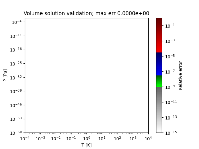
static volume_solutions_mp(T, P, b, delta, epsilon, a_alpha, dps=50)

Solution of this form of the cubic EOS in terms of volumes, using the mpmath arbitrary precision library. The number of decimal places returned is controlled by the dps parameter.

This function is the reference implementation which provides exactly correct solutions; other algorithms are compared against this one.

Parameters

Tfloat

Temperature, [K]

Pfloat

Pressure, [Pa]

bfloat

Coefficient calculated by EOS-specific method, [m^3/mol]

deltafloat

Coefficient calculated by EOS-specific method, [m^3/mol]

epsilonfloat

Coefficient calculated by EOS-specific method, [m^6/mol^2]

a_alphafloat

Coefficient calculated by EOS-specific method, [J^2/mol^2/Pa]

dpsint

Number of decimal places in the result by mpmath, [-]

Returns

Vstuple[complex]

Three possible molar volumes, [m^3/mol]

Notes

Although mpmath has a cubic solver, it has been found to fail to solve in some cases. Accordingly, the algorithm is as follows:

Working precision is dps plus 40 digits; and if P < 1e-10 Pa, it is dps plus 400 digits. The input parameters are converted exactly to mpf objects on input.

polyroots from mpmath is used with maxsteps=2000, and extra precision of 15 digits. If the solution does not converge, 20 extra digits are added up to 8 times. If no solution is found, mpmath’s findroot is called on the pressure error function using three initial guesses from another solver.

Needless to say, this function is quite slow.

References

1

Johansson, Fredrik. Mpmath: A Python Library for Arbitrary-Precision Floating-Point Arithmetic, 2010.

Examples

Test case which presented issues for PR EOS (three roots were not being returned):

>>> volume_solutions_mpmath(0.01, 1e-05, 2.5405184201558786e-05, 5.081036840311757e-05, -6.454233843151321e-10, 0.3872747173781095)
(mpf('0.0000254054613415548712260258773060137'), mpf('4.66038025602155259976574392093252'), mpf('8309.80218708657190094424659859346'))

Standard Peng-Robinson Family EOSs

Standard Peng Robinson

class thermo.eos.PR(Tc, Pc, omega, T=None, P=None, V=None)

Bases: thermo.eos.GCEOS

Class for solving the Peng-Robinson [1] [2] cubic equation of state for a pure compound. Subclasses GCEOS, which provides the methods for solving the EOS and calculating its assorted relevant thermodynamic properties. Solves the EOS on initialization.

The main methods here are PR.a_alpha_and_derivatives_pure, which calculates $a \alpha$ and its first and second derivatives, and PR.solve_T, which from a specified P and V obtains T.

Two of (T, P, V) are needed to solve the EOS.

$$P = \frac{RT}{v-b}-\frac{a\alpha(T)}{v(v+b)+b(v-b)}$$

$$a=0.45724\frac{R^2T_c^2}{P_c}$$

$$b=0.07780\frac{RT_c}{P_c}$$

$$\alpha(T)=[1+\kappa(1-\sqrt{T_r})]^2$$

$$\kappa=0.37464+1.54226\omega-0.26992\omega^2$$

Parameters

Tcfloat

Critical temperature, [K]

Pcfloat

Critical pressure, [Pa]

omegafloat

Acentric factor, [-]

Tfloat, optional

Temperature, [K]

Pfloat, optional

Pressure, [Pa]

Vfloat, optional

Molar volume, [m^3/mol]

Notes

The constants in the expresions for a and b are given to full precision in the actual code, as derived in [3].

The full expression for critical compressibility is:

$$Z_c = \frac{1}{32} \left(\sqrt[3]{16 \sqrt{2}-13}-\frac{7}{\sqrt[3] {16 \sqrt{2}-13}}+11\right)$$

References

1

Peng, Ding-Yu, and Donald B. Robinson. “A New Two-Constant Equation of State.” Industrial & Engineering Chemistry Fundamentals 15, no. 1 (February 1, 1976): 59-64. doi:10.1021/i160057a011.

2

Robinson, Donald B., Ding-Yu Peng, and Samuel Y-K Chung. “The Development of the Peng - Robinson Equation and Its Application to Phase Equilibrium in a System Containing Methanol.” Fluid Phase Equilibria 24, no. 1 (January 1, 1985): 25-41. doi:10.1016/0378-3812(85)87035-7.

3

Privat, R., and J.-N. Jaubert. “PPR78, a Thermodynamic Model for the Prediction of Petroleum Fluid-Phase Behaviour,” 11. EDP Sciences, 2011. doi:10.1051/jeep/201100011.

Examples

T-P initialization, and exploring each phase’s properties:

>>> eos = PR(Tc=507.6, Pc=3025000.0, omega=0.2975, T=400., P=1E6)
>>> eos.V_l, eos.V_g
(0.000156073184785, 0.0021418768167)
>>> eos.phase
'l/g'
>>> eos.H_dep_l, eos.H_dep_g
(-26111.8775716, -3549.30057795)
>>> eos.S_dep_l, eos.S_dep_g
(-58.098447843, -6.4394518931)
>>> eos.U_dep_l, eos.U_dep_g
(-22942.1657091, -2365.3923474)
>>> eos.G_dep_l, eos.G_dep_g
(-2872.49843435, -973.51982071)
>>> eos.A_dep_l, eos.A_dep_g
(297.21342811, 210.38840980)
>>> eos.beta_l, eos.beta_g
(0.00269337091778, 0.0101232239111)
>>> eos.kappa_l, eos.kappa_g
(9.3357215438e-09, 1.97106698097e-06)
>>> eos.Cp_minus_Cv_l, eos.Cp_minus_Cv_g
(48.510162249, 44.544161128)
>>> eos.Cv_dep_l, eos.Cp_dep_l
(18.8921126734, 59.0878123050)

P-T initialization, liquid phase, and round robin trip:

>>> eos = PR(Tc=507.6, Pc=3025000, omega=0.2975, T=299., P=1E6)
>>> eos.phase, eos.V_l, eos.H_dep_l, eos.S_dep_l
('l', 0.000130222125139, -31134.75084, -72.47561931)

T-V initialization, liquid phase:

>>> eos2 = PR(Tc=507.6, Pc=3025000, omega=0.2975, T=299., V=eos.V_l)
>>> eos2.P, eos2.phase
(1000000.00, 'l')

P-V initialization at same state:

>>> eos3 = PR(Tc=507.6, Pc=3025000, omega=0.2975, V=eos.V_l, P=1E6)
>>> eos3.T, eos3.phase
(299.0000000000, 'l')

Methods

P_max_at_V(V)	Method to calculate the maximum pressure the EOS can create at a constant volume, if one exists; returns None otherwise.
a_alpha_and_derivatives_pure(T)	Method to calculate $a \alpha$ and its first and second derivatives for this EOS.
a_alpha_pure(T)	Method to calculate $a \alpha$ for this EOS.
d3a_alpha_dT3_pure(T)	Method to calculate the third temperature derivative of a_alpha.
solve_T(P, V[, solution])	Method to calculate T from a specified P and V for the PR EOS.

P_max_at_V(V)

Method to calculate the maximum pressure the EOS can create at a constant volume, if one exists; returns None otherwise.

Parameters

Vfloat

Constant molar volume, [m^3/mol]

Returns

Pfloat

Maximum possible isochoric pressure, [Pa]

Notes

The analytical determination of this formula involved some part of the discriminant, and much black magic.

Examples

>>> e = PR(P=1e5, V=0.0001437, Tc=512.5, Pc=8084000.0, omega=0.559)
>>> e.P_max_at_V(e.V)
2247886208.7

Zc = 0.30740130869870386

Mechanical compressibility of Peng-Robinson EOS

a_alpha_and_derivatives_pure(T)

Method to calculate $a \alpha$ and its first and second derivatives for this EOS. Uses the set values of Tc, kappa, and a.

$$a\alpha = a \left(\kappa \left(- \frac{T^{0.5}}{Tc^{0.5}} + 1\right) + 1\right)^{2}$$

$$\frac{d a\alpha}{dT} = - \frac{1.0 a \kappa}{T^{0.5} Tc^{0.5}} \left(\kappa \left(- \frac{T^{0.5}}{Tc^{0.5}} + 1\right) + 1\right)$$

$$\frac{d^2 a\alpha}{dT^2} = 0.5 a \kappa \left(- \frac{1}{T^{1.5} Tc^{0.5}} \left(\kappa \left(\frac{T^{0.5}}{Tc^{0.5}} - 1\right) - 1\right) + \frac{\kappa}{T^{1.0} Tc^{1.0}}\right)$$

Parameters

Tfloat

Temperature at which to calculate the values, [-]

Returns

a_alphafloat

Coefficient calculated by EOS-specific method, [J^2/mol^2/Pa]

da_alpha_dTfloat

Temperature derivative of coefficient calculated by EOS-specific method, [J^2/mol^2/Pa/K]

d2a_alpha_dT2float

Second temperature derivative of coefficient calculated by EOS-specific method, [J^2/mol^2/Pa/K^2]

Notes

This method does not alter the object’s state and the temperature provided can be a different than that of the object.

Examples

Dodecane at 250 K:

>>> eos = PR(Tc=658.0, Pc=1820000.0, omega=0.562, T=500., P=1e5)
>>> eos.a_alpha_and_derivatives_pure(250.0)
(15.66839156301, -0.03094091246957, 9.243186769880e-05)

a_alpha_pure(T)

Method to calculate $a \alpha$ for this EOS. Uses the set values of Tc, kappa, and a.

$$a\alpha = a \left(\kappa \left(- \frac{T^{0.5}}{Tc^{0.5}} + 1\right) + 1\right)^{2}$$

Parameters

Tfloat

Temperature at which to calculate the value, [-]

Returns

a_alphafloat

Coefficient calculated by EOS-specific method, [J^2/mol^2/Pa]

Notes

This method does not alter the object’s state and the temperature provided can be a different than that of the object.

Examples

Dodecane at 250 K:

>>> eos = PR(Tc=658.0, Pc=1820000.0, omega=0.562, T=500., P=1e5)
>>> eos.a_alpha_pure(250.0)
15.66839156301

c1 = 0.4572355289213822

Full value of the constant in the a parameter

c2 = 0.07779607390388846

Full value of the constant in the b parameter

d3a_alpha_dT3_pure(T)

Method to calculate the third temperature derivative of a_alpha. Uses the set values of Tc, kappa, and a. This property is not normally needed.

$$\frac{d^3 a\alpha}{dT^3} = \frac{3 a\kappa \left(- \frac{\kappa} {T_{c}} + \frac{\sqrt{\frac{T}{T_{c}}} \left(\kappa \left(\sqrt{\frac{T} {T_{c}}} - 1\right) - 1\right)}{T}\right)}{4 T^{2}}$$

Parameters

Tfloat

Temperature at which to calculate the derivative, [-]

Returns

d3a_alpha_dT3float

Third temperature derivative of coefficient calculated by EOS-specific method, [J^2/mol^2/Pa/K^3]

Notes

This method does not alter the object’s state and the temperature provided can be a different than that of the object.

Examples

Dodecane at 500 K:

>>> eos = PR(Tc=658.0, Pc=1820000.0, omega=0.562, T=500., P=1e5)
>>> eos.d3a_alpha_dT3_pure(500.0)
-9.8038800671e-08

solve_T(P, V, solution=None)

Method to calculate T from a specified P and V for the PR EOS. Uses Tc, a, b, and kappa as well, obtained from the class’s namespace.

Parameters

Pfloat

Pressure, [Pa]

Vfloat

Molar volume, [m^3/mol]

solutionstr or None, optional

‘l’ or ‘g’ to specify a liquid of vapor solution (if one exists); if None, will select a solution more likely to be real (closer to STP, attempting to avoid temperatures like 60000 K or 0.0001 K).

Returns

Tfloat

Temperature, [K]

Notes

The exact solution can be derived as follows, and is excluded for breviety.

>>> from sympy import *
>>> P, T, V = symbols('P, T, V')
>>> Tc, Pc, omega = symbols('Tc, Pc, omega')
>>> R, a, b, kappa = symbols('R, a, b, kappa')
>>> a_alpha = a*(1 + kappa*(1-sqrt(T/Tc)))**2
>>> PR_formula = R*T/(V-b) - a_alpha/(V*(V+b)+b*(V-b)) - P
>>> #solve(PR_formula, T)

After careful evaluation of the results of the analytical formula, it was discovered, that numerical precision issues required several NR refinement iterations; at at times, when the analytical value is extremely erroneous, a call to a full numerical solver not using the analytical solution at all is required.

Examples

>>> eos = PR(Tc=658.0, Pc=1820000.0, omega=0.562, T=500., P=1e5)
>>> eos.solve_T(P=eos.P, V=eos.V_g)
500.0000000

Peng Robinson (1978)

class thermo.eos.PR78(Tc, Pc, omega, T=None, P=None, V=None)

Bases: thermo.eos.PR

Class for solving the Peng-Robinson cubic equation of state for a pure compound according to the 1978 variant [1] [2]. Subclasses PR, which provides everything except the variable kappa. Solves the EOS on initialization. See PR for further documentation.

$$P = \frac{RT}{v-b}-\frac{a\alpha(T)}{v(v+b)+b(v-b)}$$

$$a=0.45724\frac{R^2T_c^2}{P_c}$$

$$b=0.07780\frac{RT_c}{P_c}$$

$$\alpha(T)=[1+\kappa(1-\sqrt{T_r})]^2$$

$$\kappa_i = 0.37464+1.54226\omega_i-0.26992\omega_i^2 \text{ if } \omega_i \le 0.491$$

$$\kappa_i = 0.379642 + 1.48503 \omega_i - 0.164423\omega_i^2 + 0.016666 \omega_i^3 \text{ if } \omega_i > 0.491$$

Parameters

Tcfloat

Critical temperature, [K]

Pcfloat

Critical pressure, [Pa]

omegafloat

Acentric factor, [-]

Tfloat, optional

Temperature, [K]

Pfloat, optional

Pressure, [Pa]

Vfloat, optional

Molar volume, [m^3/mol]

Notes

This variant is recommended over the original.

References

1

Robinson, Donald B, and Ding-Yu Peng. The Characterization of the Heptanes and Heavier Fractions for the GPA Peng-Robinson Programs. Tulsa, Okla.: Gas Processors Association, 1978.

2

Robinson, Donald B., Ding-Yu Peng, and Samuel Y-K Chung. “The Development of the Peng - Robinson Equation and Its Application to Phase Equilibrium in a System Containing Methanol.” Fluid Phase Equilibria 24, no. 1 (January 1, 1985): 25-41. doi:10.1016/0378-3812(85)87035-7.

Examples

P-T initialization (furfuryl alcohol), liquid phase:

>>> eos = PR78(Tc=632, Pc=5350000, omega=0.734, T=299., P=1E6)
>>> eos.phase, eos.V_l, eos.H_dep_l, eos.S_dep_l
('l', 8.3519628969e-05, -63764.671093, -130.737153225)

high_omega_constants = (0.379642, 1.48503, -0.164423, 0.016666)

Constants for the kappa formula for the high-omega region.

low_omega_constants = (0.37464, 1.54226, -0.26992)

Constants for the kappa formula for the low-omega region.

Peng Robinson Stryjek-Vera

class thermo.eos.PRSV(Tc, Pc, omega, T=None, P=None, V=None, kappa1=None)

Bases: thermo.eos.PR

Class for solving the Peng-Robinson-Stryjek-Vera equations of state for a pure compound as given in [1]. The same as the Peng-Robinson EOS, except with a different kappa formula and with an optional fit parameter. Subclasses PR, which provides only several constants. See PR for further documentation and examples.

$$P = \frac{RT}{v-b}-\frac{a\alpha(T)}{v(v+b)+b(v-b)}$$

$$a=0.45724\frac{R^2T_c^2}{P_c}$$

$$b=0.07780\frac{RT_c}{P_c}$$

$$\alpha(T)=[1+\kappa(1-\sqrt{T_r})]^2$$

$$\kappa = \kappa_0 + \kappa_1(1 + T_r^{0.5})(0.7 - T_r)$$

$$\kappa_0 = 0.378893 + 1.4897153\omega - 0.17131848\omega^2 + 0.0196554\omega^3$$

Parameters

Tcfloat

Critical temperature, [K]

Pcfloat

Critical pressure, [Pa]

omegafloat

Acentric factor, [-]

Tfloat, optional

Temperature, [K]

Pfloat, optional

Pressure, [Pa]

Vfloat, optional

Molar volume, [m^3/mol]

kappa1float, optional

Fit parameter; available in [1] for over 90 compounds, [-]

Notes

[1] recommends that kappa1 be set to 0 for Tr > 0.7. This is not done by default; the class boolean kappa1_Tr_limit may be set to True and the problem re-solved with that specified if desired. kappa1_Tr_limit is not supported for P-V inputs.

Solutions for P-V solve for T with SciPy’s newton solver, as there is no analytical solution for T

[2] and [3] are two more resources documenting the PRSV EOS. [4] lists kappa values for 69 additional compounds. See also PRSV2. Note that tabulated kappa values should be used with the critical parameters used in their fits. Both [1] and [4] only considered vapor pressure in fitting the parameter.

References

1(1,2,3,4,5)

Stryjek, R., and J. H. Vera. “PRSV: An Improved Peng-Robinson Equation of State for Pure Compounds and Mixtures.” The Canadian Journal of Chemical Engineering 64, no. 2 (April 1, 1986): 323-33. doi:10.1002/cjce.5450640224.

2

Stryjek, R., and J. H. Vera. “PRSV - An Improved Peng-Robinson Equation of State with New Mixing Rules for Strongly Nonideal Mixtures.” The Canadian Journal of Chemical Engineering 64, no. 2 (April 1, 1986): 334-40. doi:10.1002/cjce.5450640225.

3

Stryjek, R., and J. H. Vera. “Vapor-liquid Equilibrium of Hydrochloric Acid Solutions with the PRSV Equation of State.” Fluid Phase Equilibria 25, no. 3 (January 1, 1986): 279-90. doi:10.1016/0378-3812(86)80004-8.

4(1,2)

Proust, P., and J. H. Vera. “PRSV: The Stryjek-Vera Modification of the Peng-Robinson Equation of State. Parameters for Other Pure Compounds of Industrial Interest.” The Canadian Journal of Chemical Engineering 67, no. 1 (February 1, 1989): 170-73. doi:10.1002/cjce.5450670125.

Examples

P-T initialization (hexane, with fit parameter in [1]), liquid phase:

>>> eos = PRSV(Tc=507.6, Pc=3025000, omega=0.2975, T=299., P=1E6, kappa1=0.05104)
>>> eos.phase, eos.V_l, eos.H_dep_l, eos.S_dep_l
('l', 0.000130126913554, -31698.926746, -74.16751538)

Methods

a_alpha_and_derivatives_pure(T)	Method to calculate $a \alpha$ and its first and second derivatives for this EOS.
a_alpha_pure(T)	Method to calculate $a \alpha$ for this EOS.
solve_T(P, V[, solution])	Method to calculate T from a specified P and V for the PRSV EOS.

a_alpha_and_derivatives_pure(T)

Method to calculate $a \alpha$ and its first and second derivatives for this EOS. Uses the set values of Tc, kappa0, kappa1, and a.

The a_alpha function is shown below; the first and second derivatives are not shown for brevity.

$$a\alpha = a \left(\left(\kappa_{0} + \kappa_{1} \left(\sqrt{\frac{ T}{T_{c}}} + 1\right) \left(- \frac{T}{T_{c}} + \frac{7}{10}\right) \right) \left(- \sqrt{\frac{T}{T_{c}}} + 1\right) + 1\right)^{2}$$

Parameters

Tfloat

Temperature at which to calculate the values, [-]

Returns

a_alphafloat

Coefficient calculated by EOS-specific method, [J^2/mol^2/Pa]

da_alpha_dTfloat

Temperature derivative of coefficient calculated by EOS-specific method, [J^2/mol^2/Pa/K]

d2a_alpha_dT2float

Second temperature derivative of coefficient calculated by EOS-specific method, [J^2/mol^2/Pa/K^2]

Notes

This method does not alter the object’s state and the temperature provided can be a different than that of the object.

The expressions can be derived as follows:

>>> from sympy import *
>>> P, T, V = symbols('P, T, V')
>>> Tc, Pc, omega = symbols('Tc, Pc, omega')
>>> R, a, b, kappa0, kappa1 = symbols('R, a, b, kappa0, kappa1')
>>> kappa = kappa0 + kappa1*(1 + sqrt(T/Tc))*(Rational(7, 10)-T/Tc)
>>> a_alpha = a*(1 + kappa*(1-sqrt(T/Tc)))**2
>>> # diff(a_alpha, T)
>>> # diff(a_alpha, T, 2)

Examples

>>> eos = PRSV(Tc=507.6, Pc=3025000, omega=0.2975, T=406.08, P=1E6, kappa1=0.05104)
>>> eos.a_alpha_and_derivatives_pure(185.0)
(4.76865472591, -0.0101408587212, 3.9138298092e-05)

a_alpha_pure(T)

Method to calculate $a \alpha$ for this EOS. Uses the set values of Tc, kappa0, kappa1, and a.

$$a\alpha = a \left(\left(\kappa_{0} + \kappa_{1} \left(\sqrt{\frac{ T}{T_{c}}} + 1\right) \left(- \frac{T}{T_{c}} + \frac{7}{10}\right) \right) \left(- \sqrt{\frac{T}{T_{c}}} + 1\right) + 1\right)^{2}$$

Parameters

Tfloat

Temperature at which to calculate the value, [-]

Returns

a_alphafloat

Coefficient calculated by EOS-specific method, [J^2/mol^2/Pa]

Notes

This method does not alter the object’s state and the temperature provided can be a different than that of the object.

Examples

>>> eos = PRSV(Tc=507.6, Pc=3025000, omega=0.2975, T=406.08, P=1E6, kappa1=0.05104)
>>> eos.a_alpha_pure(185.0)
4.7686547259

solve_T(P, V, solution=None)

Method to calculate T from a specified P and V for the PRSV EOS. Uses Tc, a, b, kappa0 and kappa as well, obtained from the class’s namespace.

Parameters

Pfloat

Pressure, [Pa]

Vfloat

Molar volume, [m^3/mol]

solutionstr or None, optional

‘l’ or ‘g’ to specify a liquid of vapor solution (if one exists); if None, will select a solution more likely to be real (closer to STP, attempting to avoid temperatures like 60000 K or 0.0001 K).

Returns

Tfloat

Temperature, [K]

Notes

Not guaranteed to produce a solution. There are actually two solution, one much higher than normally desired; it is possible the solver could converge on this.

Peng Robinson Stryjek-Vera 2

class thermo.eos.PRSV2(Tc, Pc, omega, T=None, P=None, V=None, kappa1=0, kappa2=0, kappa3=0)

Bases: thermo.eos.PR

Class for solving the Peng-Robinson-Stryjek-Vera 2 equations of state for a pure compound as given in [1]. The same as the Peng-Robinson EOS, except with a different kappa formula and with three fit parameters. Subclasses PR, which provides only several constants. See PR for further documentation and examples.

$$P = \frac{RT}{v-b}-\frac{a\alpha(T)}{v(v+b)+b(v-b)}$$

$$a=0.45724\frac{R^2T_c^2}{P_c}$$

$$b=0.07780\frac{RT_c}{P_c}$$

$$\alpha(T)=[1+\kappa(1-\sqrt{T_r})]^2$$

$$\kappa = \kappa_0 + [\kappa_1 + \kappa_2(\kappa_3 - T_r)(1-T_r^{0.5})] (1 + T_r^{0.5})(0.7 - T_r)$$

$$\kappa_0 = 0.378893 + 1.4897153\omega - 0.17131848\omega^2 + 0.0196554\omega^3$$

Parameters

Tcfloat

Critical temperature, [K]

Pcfloat

Critical pressure, [Pa]

omegafloat

Acentric factor, [-]

Tfloat, optional

Temperature, [K]

Pfloat, optional

Pressure, [Pa]

Vfloat, optional

Molar volume, [m^3/mol]

kappa1float, optional

Fit parameter; available in [1] for over 90 compounds, [-]

kappa2float, optional

Fit parameter; available in [1] for over 90 compounds, [-]

kappafloat, optional

Fit parameter; available in [1] for over 90 compounds, [-]

Notes

Note that tabulated kappa values should be used with the critical parameters used in their fits. [1] considered only vapor pressure in fitting the parameter.

References

1(1,2,3,4,5,6)

Stryjek, R., and J. H. Vera. “PRSV2: A Cubic Equation of State for Accurate Vapor-liquid Equilibria Calculations.” The Canadian Journal of Chemical Engineering 64, no. 5 (October 1, 1986): 820-26. doi:10.1002/cjce.5450640516.

Examples

P-T initialization (hexane, with fit parameter in [1]), liquid phase:

>>> eos = PRSV2(Tc=507.6, Pc=3025000, omega=0.2975, T=299., P=1E6, kappa1=0.05104, kappa2=0.8634, kappa3=0.460)
>>> eos.phase, eos.V_l, eos.H_dep_l, eos.S_dep_l
('l', 0.000130188257591, -31496.1841687, -73.615282963)

Methods

a_alpha_and_derivatives_pure(T)	Method to calculate $a \alpha$ and its first and second derivatives for this EOS.
a_alpha_pure(T)	Method to calculate $a \alpha$ for this EOS.
solve_T(P, V[, solution])	Method to calculate T from a specified P and V for the PRSV2 EOS.

a_alpha_and_derivatives_pure(T)

Method to calculate $a \alpha$ and its first and second derivatives for this EOS. Uses the set values of Tc, kappa0, kappa1, kappa2, kappa3, and a.

$$\alpha(T)=[1+\kappa(1-\sqrt{T_r})]^2$$

$$\kappa = \kappa_0 + [\kappa_1 + \kappa_2(\kappa_3 - T_r)(1-T_r^{0.5})] (1 + T_r^{0.5})(0.7 - T_r)$$

Parameters

Tfloat

Temperature at which to calculate the values, [-]

Returns

a_alphafloat

Coefficient calculated by EOS-specific method, [J^2/mol^2/Pa]

da_alpha_dTfloat

Temperature derivative of coefficient calculated by EOS-specific method, [J^2/mol^2/Pa/K]

d2a_alpha_dT2float

Second temperature derivative of coefficient calculated by EOS-specific method, [J^2/mol^2/Pa/K^2]

Notes

The first and second derivatives of a_alpha are available through the following SymPy expression.

>>> from sympy import *  
>>> P, T, V = symbols('P, T, V')  
>>> Tc, Pc, omega = symbols('Tc, Pc, omega')  
>>> R, a, b, kappa0, kappa1, kappa2, kappa3 = symbols('R, a, b, kappa0, kappa1, kappa2, kappa3')  
>>> Tr = T/Tc  
>>> kappa = kappa0 + (kappa1 + kappa2*(kappa3-Tr)*(1-sqrt(Tr)))*(1+sqrt(Tr))*(Rational('0.7')-Tr)  
>>> a_alpha = a*(1 + kappa*(1-sqrt(T/Tc)))**2  
>>> diff(a_alpha, T)  
>>> diff(a_alpha, T, 2)  

Examples

>>> eos = PRSV2(Tc=507.6, Pc=3025000, omega=0.2975, T=400., P=1E6, kappa1=0.05104, kappa2=0.8634, kappa3=0.460)
>>> eos.a_alpha_and_derivatives_pure(311.0)
(3.7245418495, -0.0066115440470, 2.05871011677e-05)

a_alpha_pure(T)

Method to calculate $a \alpha$ for this EOS. Uses the set values of Tc, kappa0, kappa1, kappa2, kappa3, and a.

$$\alpha(T)=[1+\kappa(1-\sqrt{T_r})]^2$$

$$\kappa = \kappa_0 + [\kappa_1 + \kappa_2(\kappa_3 - T_r)(1-T_r^{0.5})] (1 + T_r^{0.5})(0.7 - T_r)$$

Parameters

Tfloat

Temperature at which to calculate the values, [-]

Returns

a_alphafloat

Coefficient calculated by EOS-specific method, [J^2/mol^2/Pa]

Examples

>>> eos = PRSV2(Tc=507.6, Pc=3025000, omega=0.2975, T=400., P=1E6, kappa1=0.05104, kappa2=0.8634, kappa3=0.460)
>>> eos.a_alpha_pure(1276.0)
33.321674050

solve_T(P, V, solution=None)

Method to calculate T from a specified P and V for the PRSV2 EOS. Uses Tc, a, b, kappa0, kappa1, kappa2, and kappa3 as well, obtained from the class’s namespace.

Parameters

Pfloat

Pressure, [Pa]

Vfloat

Molar volume, [m^3/mol]

solutionstr or None, optional

‘l’ or ‘g’ to specify a liquid of vapor solution (if one exists); if None, will select a solution more likely to be real (closer to STP, attempting to avoid temperatures like 60000 K or 0.0001 K).

Returns

Tfloat

Temperature, [K]

Notes

Not guaranteed to produce a solution. There are actually 8 solutions, six with an imaginary component at a tested point. The two temperature solutions are quite far apart, with one much higher than the other; it is possible the solver could converge on the higher solution, so use T inputs with care. This extra solution is a perfectly valid one however. The secant method is implemented at present.

Examples

>>> eos = PRSV2(Tc=507.6, Pc=3025000, omega=0.2975, T=400., P=1E6, kappa1=0.05104, kappa2=0.8634, kappa3=0.460)
>>> eos.solve_T(P=eos.P, V=eos.V_g)
400.0

Peng Robinson Twu (1995)

class thermo.eos.TWUPR(Tc, Pc, omega, T=None, P=None, V=None)

Bases: thermo.eos_alpha_functions.TwuPR95_a_alpha, thermo.eos.PR

Class for solving the Twu (1995) [1] variant of the Peng-Robinson cubic equation of state for a pure compound. Subclasses PR, which provides the methods for solving the EOS and calculating its assorted relevant thermodynamic properties. Solves the EOS on initialization.

The main implemented method here is a_alpha_and_derivatives_pure, which sets $a \alpha$ and its first and second derivatives.

Two of T, P, and V are needed to solve the EOS.

$$P = \frac{RT}{v-b}-\frac{a\alpha(T)}{v(v+b)+b(v-b)}$$

$$a=0.45724\frac{R^2T_c^2}{P_c}$$

$$b=0.07780\frac{RT_c}{P_c}$$

$$\alpha = \alpha^{(0)} + \omega(\alpha^{(1)}-\alpha^{(0)})$$

$$\alpha^{(i)} = T_r^{N(M-1)}\exp[L(1-T_r^{NM})]$$

For sub-critical conditions:

L0, M0, N0 = 0.125283, 0.911807, 1.948150;

L1, M1, N1 = 0.511614, 0.784054, 2.812520

For supercritical conditions:

L0, M0, N0 = 0.401219, 4.963070, -0.2;

L1, M1, N1 = 0.024955, 1.248089, -8.

Parameters

Tcfloat

Critical temperature, [K]

Pcfloat

Critical pressure, [Pa]

omegafloat

Acentric factor, [-]

Tfloat, optional

Temperature, [K]

Pfloat, optional

Pressure, [Pa]

Vfloat, optional

Molar volume, [m^3/mol]

Notes

Claimed to be more accurate than the PR, PR78 and PRSV equations.

There is no analytical solution for T. There are multiple possible solutions for T under certain conditions; no guaranteed are provided regarding which solution is obtained.

References

1

Twu, Chorng H., John E. Coon, and John R. Cunningham. “A New Generalized Alpha Function for a Cubic Equation of State Part 1. Peng-Robinson Equation.” Fluid Phase Equilibria 105, no. 1 (March 15, 1995): 49-59. doi:10.1016/0378-3812(94)02601-V.

Examples

>>> eos = TWUPR(Tc=507.6, Pc=3025000, omega=0.2975, T=299., P=1E6)
>>> eos.V_l, eos.H_dep_l, eos.S_dep_l
(0.00013017554170, -31652.73712, -74.112850429)

Methods

a_alpha_and_derivatives_pure(T)	Method to calculate $a \alpha$ and its first and second derivatives for the Twu alpha function.
a_alpha_pure(T)	Method to calculate $a \alpha$ for the Twu alpha function.

a_alpha_and_derivatives_pure(T)

Method to calculate $a \alpha$ and its first and second derivatives for the Twu alpha function. Uses the set values of Tc, omega and a.

$$\alpha = \alpha^{(0)} + \omega(\alpha^{(1)}-\alpha^{(0)})$$

$$\alpha^{(i)} = T_r^{N(M-1)}\exp[L(1-T_r^{NM})]$$

For sub-critical conditions:

L0, M0, N0 = 0.125283, 0.911807, 1.948150;

L1, M1, N1 = 0.511614, 0.784054, 2.812520

For supercritical conditions:

L0, M0, N0 = 0.401219, 4.963070, -0.2;

L1, M1, N1 = 0.024955, 1.248089, -8.

Parameters

Tfloat

Temperature at which to calculate the values, [-]

Returns

a_alphafloat

Coefficient calculated by EOS-specific method, [J^2/mol^2/Pa]

da_alpha_dTfloat

Temperature derivative of coefficient calculated by EOS-specific method, [J^2/mol^2/Pa/K]

d2a_alpha_dT2float

Second temperature derivative of coefficient calculated by EOS-specific method, [J^2/mol^2/Pa/K^2]

Notes

This method does not alter the object’s state and the temperature provided can be a different than that of the object.

The derivatives are somewhat long and are not described here for brevity; they are obtainable from the following SymPy expression.

>>> from sympy import *   
>>> T, Tc, omega, N1, N0, M1, M0, L1, L0 = symbols('T, Tc, omega, N1, N0, M1, M0, L1, L0')  
>>> Tr = T/Tc  
>>> alpha0 = Tr**(N0*(M0-1))*exp(L0*(1-Tr**(N0*M0)))  
>>> alpha1 = Tr**(N1*(M1-1))*exp(L1*(1-Tr**(N1*M1)))  
>>> alpha = alpha0 + omega*(alpha1-alpha0)  
>>> diff(alpha, T)  
>>> diff(alpha, T, T)  

a_alpha_pure(T)

Method to calculate $a \alpha$ for the Twu alpha function. Uses the set values of Tc, omega and a.

$$\alpha = \alpha^{(0)} + \omega(\alpha^{(1)}-\alpha^{(0)})$$

$$\alpha^{(i)} = T_r^{N(M-1)}\exp[L(1-T_r^{NM})]$$

For sub-critical conditions:

L0, M0, N0 = 0.125283, 0.911807, 1.948150;

L1, M1, N1 = 0.511614, 0.784054, 2.812520

For supercritical conditions:

L0, M0, N0 = 0.401219, 4.963070, -0.2;

L1, M1, N1 = 0.024955, 1.248089, -8.

Parameters

Tfloat

Temperature at which to calculate the value, [-]

Returns

a_alphafloat

Coefficient calculated by EOS-specific method, [J^2/mol^2/Pa]

Notes

This method does not alter the object’s state and the temperature provided can be a different than that of the object.

Peng Robinson Polynomial alpha Function

class thermo.eos.PRTranslatedPoly(Tc, Pc, omega, alpha_coeffs=None, c=0.0, T=None, P=None, V=None)

Bases: thermo.eos_alpha_functions.Poly_a_alpha, thermo.eos.PRTranslated

Class for solving the volume translated Peng-Robinson equation of state with a polynomial alpha function. With the right coefficients, this model can reproduce any property incredibly well. Subclasses PRTranslated. Solves the EOS on initialization. This is intended as a base class for all translated variants of the Peng-Robinson EOS.

$$P = \frac{RT}{v + c - b} - \frac{a\alpha(T)}{(v+c)(v + c + b)+b(v + c - b)}$$

$$a=0.45724\frac{R^2T_c^2}{P_c}$$

$$b=0.07780\frac{RT_c}{P_c}$$

$$\alpha(T)=f(T)$$

$$\kappa=0.37464+1.54226\omega-0.26992\omega^2$$

Parameters

Tcfloat

Critical temperature, [K]

Pcfloat

Critical pressure, [Pa]

omegafloat

Acentric factor, [-]

alpha_coeffstuple or None

Coefficients which may be specified by subclasses; set to None to use the original Peng-Robinson alpha function, [-]

cfloat, optional

Volume translation parameter, [m^3/mol]

Tfloat, optional

Temperature, [K]

Pfloat, optional

Pressure, [Pa]

Vfloat, optional

Molar volume, [m^3/mol]

Examples

Methanol, with alpha functions reproducing CoolProp’s implementation of its vapor pressure (up to 13 coefficients)

>>> alpha_coeffs_exact = [9.645280470011588e-32, -4.362226651748652e-28, 9.034194757823037e-25, -1.1343330204981244e-21, 9.632898335494218e-19, -5.841502902171077e-16, 2.601801729901228e-13, -8.615431349241052e-11, 2.1202999753932622e-08, -3.829144045293198e-06, 0.0004930777289075716, -0.04285337965522619, 2.2473964123842705, -51.13852710672087]
>>> kwargs = dict(Tc=512.5, Pc=8084000.0, omega=0.559, alpha_coeffs=alpha_coeffs_exact, c=1.557458e-05)
>>> eos = PRTranslatedPoly(T=300, P=1e5, **kwargs)
>>> eos.Psat(500)/PropsSI("P", 'T', 500.0, 'Q', 0, 'methanol') 
1.0000112765

Methods

a_alpha_and_derivatives_pure(T)	Method to calculate a_alpha and its first and second derivatives given that there is a polynomial equation for $\alpha$.
a_alpha_pure(T)	Method to calculate a_alpha given that there is a polynomial equation for $\alpha$.

a_alpha_and_derivatives_pure(T)

Method to calculate a_alpha and its first and second derivatives given that there is a polynomial equation for $\alpha$.

$$a \alpha = a\cdot \text{poly}(T)$$

Parameters

Tfloat

Temperature, [K]

Returns

a_alphaslist[float]

Coefficient calculated by EOS-specific method, [J^2/mol^2/Pa]

da_alpha_dTslist[float]

Temperature derivative of coefficient calculated by EOS-specific method, [J^2/mol^2/Pa/K]

d2a_alpha_dT2slist[float]

Second temperature derivative of coefficient calculated by EOS-specific method, [J^2/mol^2/Pa/K**2]

a_alpha_pure(T)

Method to calculate a_alpha given that there is a polynomial equation for $\alpha$.

$$a \alpha = a\cdot \text{poly}(T)$$

Parameters

Tfloat

Temperature, [K]

Returns

a_alphafloat

Coefficient calculated by EOS-specific method, [J^2/mol^2/Pa]

Volume Translated Peng-Robinson Family EOSs

Peng Robinson Translated

class thermo.eos.PRTranslated(Tc, Pc, omega, alpha_coeffs=None, c=0.0, T=None, P=None, V=None)

Bases: thermo.eos.PR

Class for solving the volume translated Peng-Robinson equation of state. Subclasses PR. Solves the EOS on initialization. This is intended as a base class for all translated variants of the Peng-Robinson EOS.

$$P = \frac{RT}{v + c - b} - \frac{a\alpha(T)}{(v+c)(v + c + b)+b(v + c - b)}$$

$$a=0.45724\frac{R^2T_c^2}{P_c}$$

$$b=0.07780\frac{RT_c}{P_c}$$

$$\alpha(T)=[1+\kappa(1-\sqrt{T_r})]^2$$

$$\kappa=0.37464+1.54226\omega-0.26992\omega^2$$

Parameters

Tcfloat

Critical temperature, [K]

Pcfloat

Critical pressure, [Pa]

omegafloat

Acentric factor, [-]

alpha_coeffstuple or None

Coefficients which may be specified by subclasses; set to None to use the original Peng-Robinson alpha function, [-]

cfloat, optional

Volume translation parameter, [m^3/mol]

Tfloat, optional

Temperature, [K]

Pfloat, optional

Pressure, [Pa]

Vfloat, optional

Molar volume, [m^3/mol]

References

1

Gmehling, Jürgen, Michael Kleiber, Bärbel Kolbe, and Jürgen Rarey. Chemical Thermodynamics for Process Simulation. John Wiley & Sons, 2019.

Examples

P-T initialization:

>>> eos = PRTranslated(T=305, P=1.1e5, Tc=512.5, Pc=8084000.0, omega=0.559, c=-1e-6)
>>> eos.phase, eos.V_l, eos.V_g
('l/g', 4.90798083711e-05, 0.0224350982488)

Peng Robinson Translated Twu (1991)

class thermo.eos.PRTranslatedTwu(Tc, Pc, omega, alpha_coeffs=None, c=0.0, T=None, P=None, V=None)

Bases: thermo.eos_alpha_functions.Twu91_a_alpha, thermo.eos.PRTranslated

Class for solving the volume translated Peng-Robinson equation of state with the Twu (1991) [1] alpha function. Subclasses thermo.eos_alpha_functions.Twu91_a_alpha and PRTranslated. Solves the EOS on initialization.

$$P = \frac{RT}{v + c - b} - \frac{a\alpha(T)}{(v+c)(v + c + b)+b(v + c - b)}$$

$$a=0.45724\frac{R^2T_c^2}{P_c}$$

$$b=0.07780\frac{RT_c}{P_c}$$

$$\alpha = \left(\frac{T}{T_{c}}\right)^{c_{3} \left(c_{2} - 1\right)} e^{c_{1} \left(- \left(\frac{T}{T_{c}} \right)^{c_{2} c_{3}} + 1\right)}$$

Parameters

Tcfloat

Critical temperature, [K]

Pcfloat

Critical pressure, [Pa]

omegafloat

Acentric factor, [-]

alpha_coeffstuple(float[3])

Coefficients L, M, N (also called C1, C2, C3) of TWU 1991 form, [-]

cfloat, optional

Volume translation parameter, [m^3/mol]

Tfloat, optional

Temperature, [K]

Pfloat, optional

Pressure, [Pa]

Vfloat, optional

Molar volume, [m^3/mol]

Notes

This variant offers substantial improvements to the PR-type EOSs - likely getting about as accurate as this form of cubic equation can get.

References

1

Twu, Chorng H., David Bluck, John R. Cunningham, and John E. Coon. “A Cubic Equation of State with a New Alpha Function and a New Mixing Rule.” Fluid Phase Equilibria 69 (December 10, 1991): 33-50. doi:10.1016/0378-3812(91)90024-2.

Examples

P-T initialization:

>>> alpha_coeffs = (0.694911381318495, 0.919907783415812, 1.70412689631515)
>>> kwargs = dict(Tc=512.5, Pc=8084000.0, omega=0.559, alpha_coeffs=alpha_coeffs, c=-1e-6)
>>> eos = PRTranslatedTwu(T=300, P=1e5, **kwargs)
>>> eos.phase, eos.V_l, eos.V_g
('l/g', 4.8918748906e-05, 0.024314406330)

Peng Robinson Translated-Consistent

class thermo.eos.PRTranslatedConsistent(Tc, Pc, omega, alpha_coeffs=None, c=None, T=None, P=None, V=None)

Bases: thermo.eos.PRTranslatedTwu

Class for solving the volume translated Le Guennec, Privat, and Jaubert revision of the Peng-Robinson equation of state for a pure compound according to [1]. Subclasses PRTranslatedTwu, which provides everything except the estimation of c and the alpha coefficients. This model’s alpha is based on the TWU 1991 model; when estimating, N is set to 2. Solves the EOS on initialization. See PRTranslated for further documentation.

$$P = \frac{RT}{v + c - b} - \frac{a\alpha(T)}{(v+c)(v + c + b)+b(v + c - b)}$$

$$a=0.45724\frac{R^2T_c^2}{P_c}$$

$$b=0.07780\frac{RT_c}{P_c}$$

$$\alpha = \left(\frac{T}{T_{c}}\right)^{c_{3} \left(c_{2} - 1\right)} e^{c_{1} \left(- \left(\frac{T}{T_{c}} \right)^{c_{2} c_{3}} + 1\right)}$$

If c is not provided, it is estimated as:

$$c =\frac{R T_c}{P_c}(0.0198\omega - 0.0065)$$

If alpha_coeffs is not provided, the parameters L and M are estimated from the acentric factor as follows:

$$L = 0.1290\omega^2 + 0.6039\omega + 0.0877$$

$$M = 0.1760\omega^2 - 0.2600\omega + 0.8884$$

Parameters

Tcfloat

Critical temperature, [K]

Pcfloat

Critical pressure, [Pa]

omegafloat

Acentric factor, [-]

alpha_coeffstuple(float[3]), optional

Coefficients L, M, N (also called C1, C2, C3) of TWU 1991 form, [-]

cfloat, optional

Volume translation parameter, [m^3/mol]

Tfloat, optional

Temperature, [K]

Pfloat, optional

Pressure, [Pa]

Vfloat, optional

Molar volume, [m^3/mol]

Notes

This variant offers substantial improvements to the PR-type EOSs - likely getting about as accurate as this form of cubic equation can get.

References

1

Le Guennec, Yohann, Romain Privat, and Jean-Noël Jaubert. “Development of the Translated-Consistent Tc-PR and Tc-RK Cubic Equations of State for a Safe and Accurate Prediction of Volumetric, Energetic and Saturation Properties of Pure Compounds in the Sub- and Super-Critical Domains.” Fluid Phase Equilibria 429 (December 15, 2016): 301-12. https://doi.org/10.1016/j.fluid.2016.09.003.

Examples

P-T initialization (methanol), liquid phase:

>>> eos = PRTranslatedConsistent(Tc=507.6, Pc=3025000, omega=0.2975, T=250., P=1E6)
>>> eos.phase, eos.V_l, eos.H_dep_l, eos.S_dep_l
('l', 0.000124374813374486, -34155.16119794619, -83.34913258614345)

Peng Robinson Translated (Pina-Martinez, Privat, and Jaubert Variant)

class thermo.eos.PRTranslatedPPJP(Tc, Pc, omega, c=0.0, T=None, P=None, V=None)

Bases: thermo.eos.PRTranslated

Class for solving the volume translated Pina-Martinez, Privat, Jaubert, and Peng revision of the Peng-Robinson equation of state for a pure compound according to [1]. Subclasses PRTranslated, which provides everything except the variable kappa. Solves the EOS on initialization. See PRTranslated for further documentation.

$$P = \frac{RT}{v + c - b} - \frac{a\alpha(T)}{(v+c)(v + c + b)+b(v + c - b)}$$

$$a=0.45724\frac{R^2T_c^2}{P_c}$$

$$b=0.07780\frac{RT_c}{P_c}$$

$$\alpha(T)=[1+\kappa(1-\sqrt{T_r})]^2$$

$$\kappa = 0.3919 + 1.4996 \omega - 0.2721\omega^2 + 0.1063\omega^3$$

Parameters

Tcfloat

Critical temperature, [K]

Pcfloat

Critical pressure, [Pa]

omegafloat

Acentric factor, [-]

cfloat, optional

Volume translation parameter, [m^3/mol]

Tfloat, optional

Temperature, [K]

Pfloat, optional

Pressure, [Pa]

Vfloat, optional

Molar volume, [m^3/mol]

Notes

This variant offers incremental improvements in accuracy only, but those can be fairly substantial for some substances.

References

1

Pina-Martinez, Andrés, Romain Privat, Jean-Noël Jaubert, and Ding-Yu Peng. “Updated Versions of the Generalized Soave a-Function Suitable for the Redlich-Kwong and Peng-Robinson Equations of State.” Fluid Phase Equilibria, December 7, 2018. https://doi.org/10.1016/j.fluid.2018.12.007.

Examples

P-T initialization (methanol), liquid phase:

>>> eos = PRTranslatedPPJP(Tc=507.6, Pc=3025000, omega=0.2975, c=0.6390E-6, T=250., P=1E6)
>>> eos.phase, eos.V_l, eos.H_dep_l, eos.S_dep_l
('l', 0.0001229231238092, -33466.2428296, -80.75610242427)

Soave-Redlich-Kwong Family EOSs

Standard SRK

class thermo.eos.SRK(Tc, Pc, omega, T=None, P=None, V=None)

Bases: thermo.eos.GCEOS

Class for solving the Soave-Redlich-Kwong [1] [2] [3] cubic equation of state for a pure compound. Subclasses GCEOS, which provides the methods for solving the EOS and calculating its assorted relevant thermodynamic properties. Solves the EOS on initialization.

Two of T, P, and V are needed to solve the EOS.

$$P = \frac{RT}{V-b} - \frac{a\alpha(T)}{V(V+b)}$$

$$a=\left(\frac{R^2(T_c)^{2}}{9(\sqrt[3]{2}-1)P_c} \right) =\frac{0.42748\cdot R^2(T_c)^{2}}{P_c}$$

$$b=\left( \frac{(\sqrt[3]{2}-1)}{3}\right)\frac{RT_c}{P_c} =\frac{0.08664\cdot R T_c}{P_c}$$

$$\alpha(T) = \left[1 + m\left(1 - \sqrt{\frac{T}{T_c}}\right)\right]^2$$

$$m = 0.480 + 1.574\omega - 0.176\omega^2$$

Parameters

Tcfloat

Critical temperature, [K]

Pcfloat

Critical pressure, [Pa]

omegafloat

Acentric factor, [-]

Tfloat, optional

Temperature, [K]

Pfloat, optional

Pressure, [Pa]

Vfloat, optional

Molar volume, [m^3/mol]

References

1

Soave, Giorgio. “Equilibrium Constants from a Modified Redlich-Kwong Equation of State.” Chemical Engineering Science 27, no. 6 (June 1972): 1197-1203. doi:10.1016/0009-2509(72)80096-4.

2

Poling, Bruce E. The Properties of Gases and Liquids. 5th edition. New York: McGraw-Hill Professional, 2000.

3

Walas, Stanley M. Phase Equilibria in Chemical Engineering. Butterworth-Heinemann, 1985.

Examples

>>> eos = SRK(Tc=507.6, Pc=3025000, omega=0.2975, T=299., P=1E6)
>>> eos.phase, eos.V_l, eos.H_dep_l, eos.S_dep_l
('l', 0.000146821077354, -31754.663859, -74.373272044)

Methods

P_max_at_V(V)	Method to calculate the maximum pressure the EOS can create at a constant volume, if one exists; returns None otherwise.
a_alpha_and_derivatives_pure(T)	Method to calculate $a \alpha$ and its first and second derivatives for this EOS.
a_alpha_pure(T)	Method to calculate $a \alpha$ for this EOS.
solve_T(P, V[, solution])	Method to calculate T from a specified P and V for the SRK EOS.

P_max_at_V(V)

Method to calculate the maximum pressure the EOS can create at a constant volume, if one exists; returns None otherwise.

Parameters

Vfloat

Constant molar volume, [m^3/mol]

Returns

Pfloat

Maximum possible isochoric pressure, [Pa]

Notes

The analytical determination of this formula involved some part of the discriminant, and much black magic.

Examples

>>> e = SRK(P=1e5, V=0.0001437, Tc=512.5, Pc=8084000.0, omega=0.559)
>>> e.P_max_at_V(e.V)
490523786.2

Zc = 0.3333333333333333

Mechanical compressibility of SRK EOS

a_alpha_and_derivatives_pure(T)

Method to calculate $a \alpha$ and its first and second derivatives for this EOS. Uses the set values of Tc, m, and a.

$$a\alpha = a \left(m \left(- \sqrt{\frac{T}{T_{c}}} + 1\right) + 1\right)^{2}$$

$$\frac{d a\alpha}{dT} = \frac{a m}{T} \sqrt{\frac{T}{T_{c}}} \left(m \left(\sqrt{\frac{T}{T_{c}}} - 1\right) - 1\right)$$

$$\frac{d^2 a\alpha}{dT^2} = \frac{a m \sqrt{\frac{T}{T_{c}}}}{2 T^{2}} \left(m + 1\right)$$

Parameters

Tfloat

Temperature at which to calculate the values, [-]

Returns

a_alphafloat

Coefficient calculated by EOS-specific method, [J^2/mol^2/Pa]

da_alpha_dTfloat

Temperature derivative of coefficient calculated by EOS-specific method, [J^2/mol^2/Pa/K]

d2a_alpha_dT2float

Second temperature derivative of coefficient calculated by EOS-specific method, [J^2/mol^2/Pa/K^2]

a_alpha_pure(T)

Method to calculate $a \alpha$ for this EOS. Uses the set values of Tc, m, and a.

$$a\alpha = a \left(m \left(- \sqrt{\frac{T}{T_{c}}} + 1\right) + 1\right)^{2}$$

Parameters

Tfloat

Temperature at which to calculate the values, [-]

Returns

a_alphafloat

Coefficient calculated by EOS-specific method, [J^2/mol^2/Pa]

c1 = 0.4274802335403414

Full value of the constant in the a parameter

c2 = 0.08664034996495772

Full value of the constant in the b parameter

epsilon = 0.0

epsilon is always zero for the SRK EOS

solve_T(P, V, solution=None)

Method to calculate T from a specified P and V for the SRK EOS. Uses a, b, and Tc obtained from the class’s namespace.

Parameters

Pfloat

Pressure, [Pa]

Vfloat

Molar volume, [m^3/mol]

solutionstr or None, optional

‘l’ or ‘g’ to specify a liquid of vapor solution (if one exists); if None, will select a solution more likely to be real (closer to STP, attempting to avoid temperatures like 60000 K or 0.0001 K).

Returns

Tfloat

Temperature, [K]

Notes

The exact solution can be derived as follows; it is excluded for breviety.

>>> from sympy import * 
>>> P, T, V, R, a, b, m = symbols('P, T, V, R, a, b, m') 
>>> Tc, Pc, omega = symbols('Tc, Pc, omega') 
>>> a_alpha = a*(1 + m*(1-sqrt(T/Tc)))**2 
>>> SRK = R*T/(V-b) - a_alpha/(V*(V+b)) - P 
>>> solve(SRK, T) 

Twu SRK (1995)

class thermo.eos.TWUSRK(Tc, Pc, omega, T=None, P=None, V=None)

Bases: thermo.eos_alpha_functions.TwuSRK95_a_alpha, thermo.eos.SRK

Class for solving the Soave-Redlich-Kwong cubic equation of state for a pure compound. Subclasses GCEOS, which provides the methods for solving the EOS and calculating its assorted relevant thermodynamic properties. Solves the EOS on initialization.

The main implemented method here is a_alpha_and_derivatives_pure, which sets $a \alpha$ and its first and second derivatives.

Two of T, P, and V are needed to solve the EOS.

$$P = \frac{RT}{V-b} - \frac{a\alpha(T)}{V(V+b)}$$

$$a=\left(\frac{R^2(T_c)^{2}}{9(\sqrt[3]{2}-1)P_c} \right) =\frac{0.42748\cdot R^2(T_c)^{2}}{P_c}$$

$$b=\left( \frac{(\sqrt[3]{2}-1)}{3}\right)\frac{RT_c}{P_c} =\frac{0.08664\cdot R T_c}{P_c}$$

$$\alpha = \alpha^{(0)} + \omega(\alpha^{(1)}-\alpha^{(0)})$$

$$\alpha^{(i)} = T_r^{N(M-1)}\exp[L(1-T_r^{NM})]$$

For sub-critical conditions:

L0, M0, N0 = 0.141599, 0.919422, 2.496441

L1, M1, N1 = 0.500315, 0.799457, 3.291790

For supercritical conditions:

L0, M0, N0 = 0.441411, 6.500018, -0.20

L1, M1, N1 = 0.032580, 1.289098, -8.0

Parameters

Tcfloat

Critical temperature, [K]

Pcfloat

Critical pressure, [Pa]

omegafloat

Acentric factor, [-]

Tfloat, optional

Temperature, [K]

Pfloat, optional

Pressure, [Pa]

Vfloat, optional

Molar volume, [m^3/mol]

Notes

There is no analytical solution for T. There are multiple possible solutions for T under certain conditions; no guaranteed are provided regarding which solution is obtained.

References

1

Twu, Chorng H., John E. Coon, and John R. Cunningham. “A New Generalized Alpha Function for a Cubic Equation of State Part 2. Redlich-Kwong Equation.” Fluid Phase Equilibria 105, no. 1 (March 15, 1995): 61-69. doi:10.1016/0378-3812(94)02602-W.

Examples

>>> eos = TWUSRK(Tc=507.6, Pc=3025000, omega=0.2975, T=299., P=1E6)
>>> eos.phase, eos.V_l, eos.H_dep_l, eos.S_dep_l
('l', 0.000146892222966, -31612.6025870, -74.022966093)

Methods

a_alpha_and_derivatives_pure(T)	Method to calculate $a \alpha$ and its first and second derivatives for the Twu alpha function.
a_alpha_pure(T)	Method to calculate $a \alpha$ for the Twu alpha function.

a_alpha_and_derivatives_pure(T)

Method to calculate $a \alpha$ and its first and second derivatives for the Twu alpha function. Uses the set values of Tc, omega and a.

$$\alpha = \alpha^{(0)} + \omega(\alpha^{(1)}-\alpha^{(0)})$$

$$\alpha^{(i)} = T_r^{N(M-1)}\exp[L(1-T_r^{NM})]$$

For sub-critical conditions:

L0, M0, N0 = 0.141599, 0.919422, 2.496441

L1, M1, N1 = 0.500315, 0.799457, 3.291790

For supercritical conditions:

L0, M0, N0 = 0.441411, 6.500018, -0.20

L1, M1, N1 = 0.032580, 1.289098, -8.0

Parameters

Tfloat

Temperature at which to calculate the values, [-]

Returns

a_alphafloat

Coefficient calculated by EOS-specific method, [J^2/mol^2/Pa]

da_alpha_dTfloat

Temperature derivative of coefficient calculated by EOS-specific method, [J^2/mol^2/Pa/K]

d2a_alpha_dT2float

Second temperature derivative of coefficient calculated by EOS-specific method, [J^2/mol^2/Pa/K^2]

Notes

This method does not alter the object’s state and the temperature provided can be a different than that of the object.

The derivatives are somewhat long and are not described here for brevity; they are obtainable from the following SymPy expression.

>>> from sympy import *   
>>> T, Tc, omega, N1, N0, M1, M0, L1, L0 = symbols('T, Tc, omega, N1, N0, M1, M0, L1, L0')  
>>> Tr = T/Tc  
>>> alpha0 = Tr**(N0*(M0-1))*exp(L0*(1-Tr**(N0*M0)))  
>>> alpha1 = Tr**(N1*(M1-1))*exp(L1*(1-Tr**(N1*M1)))  
>>> alpha = alpha0 + omega*(alpha1-alpha0)  
>>> diff(alpha, T)  
>>> diff(alpha, T, T)  

a_alpha_pure(T)

Method to calculate $a \alpha$ for the Twu alpha function. Uses the set values of Tc, omega and a.

$$\alpha = \alpha^{(0)} + \omega(\alpha^{(1)}-\alpha^{(0)})$$

$$\alpha^{(i)} = T_r^{N(M-1)}\exp[L(1-T_r^{NM})]$$

For sub-critical conditions:

L0, M0, N0 = 0.141599, 0.919422, 2.496441

L1, M1, N1 = 0.500315, 0.799457, 3.291790

For supercritical conditions:

L0, M0, N0 = 0.441411, 6.500018, -0.20

L1, M1, N1 = 0.032580, 1.289098, -8.0

Parameters

Tfloat

Temperature at which to calculate the value, [-]

Returns

a_alphafloat

Coefficient calculated by EOS-specific method, [J^2/mol^2/Pa]

Notes

This method does not alter the object’s state and the temperature provided can be a different than that of the object.

API SRK

class thermo.eos.APISRK(Tc, Pc, omega=None, T=None, P=None, V=None, S1=None, S2=0)

Bases: thermo.eos.SRK

Class for solving the Refinery Soave-Redlich-Kwong cubic equation of state for a pure compound shown in the API Databook [1]. Subclasses GCEOS, which provides the methods for solving the EOS and calculating its assorted relevant thermodynamic properties. Solves the EOS on initialization.

Implemented methods here are a_alpha_and_derivatives, which sets $a \alpha$ and its first and second derivatives, and solve_T, which from a specified P and V obtains T. Two fit constants are used in this expresion, with an estimation scheme for the first if unavailable and the second may be set to zero.

Two of T, P, and V are needed to solve the EOS.

$$P = \frac{RT}{V-b} - \frac{a\alpha(T)}{V(V+b)}$$

$$a=\left(\frac{R^2(T_c)^{2}}{9(\sqrt[3]{2}-1)P_c} \right) =\frac{0.42748\cdot R^2(T_c)^{2}}{P_c}$$

$$b=\left( \frac{(\sqrt[3]{2}-1)}{3}\right)\frac{RT_c}{P_c} =\frac{0.08664\cdot R T_c}{P_c}$$

$$\alpha(T) = \left[1 + S_1\left(1-\sqrt{T_r}\right) + S_2\frac{1 - \sqrt{T_r}}{\sqrt{T_r}}\right]^2$$

$$S_1 = 0.48508 + 1.55171\omega - 0.15613\omega^2 \text{ if S1 is not tabulated }$$

Parameters

Tcfloat

Critical temperature, [K]

Pcfloat

Critical pressure, [Pa]

omegafloat, optional

Acentric factor, [-]

Tfloat, optional

Temperature, [K]

Pfloat, optional

Pressure, [Pa]

Vfloat, optional

Molar volume, [m^3/mol]

S1float, optional

Fit constant or estimated from acentric factor if not provided [-]

S2float, optional

Fit constant or 0 if not provided [-]

References

1

API Technical Data Book: General Properties & Characterization. American Petroleum Institute, 7E, 2005.

Examples

>>> eos = APISRK(Tc=514.0, Pc=6137000.0, S1=1.678665, S2=-0.216396, P=1E6, T=299)
>>> eos.phase, eos.V_l, eos.H_dep_l, eos.S_dep_l
('l', 7.0456950702e-05, -42826.286146, -103.626979037)

Methods

a_alpha_and_derivatives_pure(T)	Method to calculate $a \alpha$ and its first and second derivatives for this EOS.
a_alpha_pure(T)	Method to calculate $a \alpha$ for this EOS.
solve_T(P, V[, solution])	Method to calculate T from a specified P and V for the API SRK EOS.

a_alpha_and_derivatives_pure(T)

Method to calculate $a \alpha$ and its first and second derivatives for this EOS. Returns a_alpha, da_alpha_dT, and d2a_alpha_dT2. See GCEOS.a_alpha_and_derivatives for more documentation. Uses the set values of Tc, a, S1, and S2.

$$a\alpha(T) = a\left[1 + S_1\left(1-\sqrt{T_r}\right) + S_2\frac{1 - \sqrt{T_r}}{\sqrt{T_r}}\right]^2$$

$$\frac{d a\alpha}{dT} = a\frac{T_{c}}{T^{2}} \left(- S_{2} \left(\sqrt{ \frac{T}{T_{c}}} - 1\right) + \sqrt{\frac{T}{T_{c}}} \left(S_{1} \sqrt{ \frac{T}{T_{c}}} + S_{2}\right)\right) \left(S_{2} \left(\sqrt{\frac{ T}{T_{c}}} - 1\right) + \sqrt{\frac{T}{T_{c}}} \left(S_{1} \left(\sqrt{ \frac{T}{T_{c}}} - 1\right) - 1\right)\right)$$

$$\frac{d^2 a\alpha}{dT^2} = a\frac{1}{2 T^{3}} \left(S_{1}^{2} T \sqrt{\frac{T}{T_{c}}} - S_{1} S_{2} T \sqrt{\frac{T}{T_{c}}} + 3 S_{1} S_{2} Tc \sqrt{\frac{T}{T_{c}}} + S_{1} T \sqrt{\frac{T}{T_{c}}} - 3 S_{2}^{2} Tc \sqrt{\frac{T}{T_{c}}} + 4 S_{2}^{2} Tc + 3 S_{2} Tc \sqrt{\frac{T}{T_{c}}}\right)$$

a_alpha_pure(T)

Method to calculate $a \alpha$ for this EOS. Uses the set values of Tc, m, and a.

$$a\alpha = a \left(m \left(- \sqrt{\frac{T}{T_{c}}} + 1\right) + 1\right)^{2}$$

Parameters

Tfloat

Temperature at which to calculate the values, [-]

Returns

a_alphafloat

Coefficient calculated by EOS-specific method, [J^2/mol^2/Pa]

solve_T(P, V, solution=None)

Method to calculate T from a specified P and V for the API SRK EOS. Uses a, b, and Tc obtained from the class’s namespace.

Parameters

Pfloat

Pressure, [Pa]

Vfloat

Molar volume, [m^3/mol]

solutionstr or None, optional

‘l’ or ‘g’ to specify a liquid of vapor solution (if one exists); if None, will select a solution more likely to be real (closer to STP, attempting to avoid temperatures like 60000 K or 0.0001 K).

Returns

Tfloat

Temperature, [K]

Notes

If S2 is set to 0, the solution is the same as in the SRK EOS, and that is used. Otherwise, newton’s method must be used to solve for T. There are 8 roots of T in that case, six of them real. No guarantee can be made regarding which root will be obtained.

SRK Translated

class thermo.eos.SRKTranslated(Tc, Pc, omega, alpha_coeffs=None, c=0.0, T=None, P=None, V=None)

Bases: thermo.eos.SRK

Class for solving the volume translated Peng-Robinson equation of state. Subclasses SRK. Solves the EOS on initialization. This is intended as a base class for all translated variants of the SRK EOS.

$$P = \frac{RT}{V + c - b} - \frac{a\alpha(T)}{(V + c)(V + c + b)}$$

$$a=\left(\frac{R^2(T_c)^{2}}{9(\sqrt[3]{2}-1)P_c} \right) =\frac{0.42748\cdot R^2(T_c)^{2}}{P_c}$$

$$b=\left( \frac{(\sqrt[3]{2}-1)}{3}\right)\frac{RT_c}{P_c} =\frac{0.08664\cdot R T_c}{P_c}$$

$$\alpha(T) = \left[1 + m\left(1 - \sqrt{\frac{T}{T_c}}\right)\right]^2$$

$$m = 0.480 + 1.574\omega - 0.176\omega^2$$

Parameters

Tcfloat

Critical temperature, [K]

Pcfloat

Critical pressure, [Pa]

omegafloat

Acentric factor, [-]

alpha_coeffstuple or None

Coefficients which may be specified by subclasses; set to None to use the original Peng-Robinson alpha function, [-]

cfloat, optional

Volume translation parameter, [m^3/mol]

Tfloat, optional

Temperature, [K]

Pfloat, optional

Pressure, [Pa]

Vfloat, optional

Molar volume, [m^3/mol]

References

1

Gmehling, Jürgen, Michael Kleiber, Bärbel Kolbe, and Jürgen Rarey. Chemical Thermodynamics for Process Simulation. John Wiley & Sons, 2019.

Examples

P-T initialization:

>>> eos = SRKTranslated(T=305, P=1.1e5, Tc=512.5, Pc=8084000.0, omega=0.559, c=-1e-6)
>>> eos.phase, eos.V_l, eos.V_g
('l/g', 5.5131657318e-05, 0.022447661363)

SRK Translated-Consistent

class thermo.eos.SRKTranslatedConsistent(Tc, Pc, omega, alpha_coeffs=None, c=None, T=None, P=None, V=None)

Bases: thermo.eos_alpha_functions.Twu91_a_alpha, thermo.eos.SRKTranslated

Class for solving the volume translated Le Guennec, Privat, and Jaubert revision of the SRK equation of state for a pure compound according to [1].

This model’s alpha is based on the TWU 1991 model; when estimating, N is set to 2. Solves the EOS on initialization. See SRK for further documentation.

$$P = \frac{RT}{V + c - b} - \frac{a\alpha(T)}{(V + c)(V + c + b)}$$

$$a=\left(\frac{R^2(T_c)^{2}}{9(\sqrt[3]{2}-1)P_c} \right) =\frac{0.42748\cdot R^2(T_c)^{2}}{P_c}$$

$$b=\left( \frac{(\sqrt[3]{2}-1)}{3}\right)\frac{RT_c}{P_c} =\frac{0.08664\cdot R T_c}{P_c}$$

$$\alpha = \left(\frac{T}{T_{c}}\right)^{c_{3} \left(c_{2} - 1\right)} e^{c_{1} \left(- \left(\frac{T}{T_{c}} \right)^{c_{2} c_{3}} + 1\right)}$$

If c is not provided, it is estimated as:

$$c =\frac{R T_c}{P_c}(0.0172\omega - 0.0096)$$

If alpha_coeffs is not provided, the parameters L and M are estimated from the acentric factor as follows:

$$L = 0.0947\omega^2 + 0.6871\omega + 0.1508$$

$$M = 0.1615\omega^2 - 0.2349\omega + 0.8876$$

Parameters

Tcfloat

Critical temperature, [K]

Pcfloat

Critical pressure, [Pa]

omegafloat

Acentric factor, [-]

alpha_coeffstuple(float[3]), optional

Coefficients L, M, N (also called C1, C2, C3) of TWU 1991 form, [-]

cfloat, optional

Volume translation parameter, [m^3/mol]

Tfloat, optional

Temperature, [K]

Pfloat, optional

Pressure, [Pa]

Vfloat, optional

Molar volume, [m^3/mol]

Notes

This variant offers substantial improvements to the SRK-type EOSs - likely getting about as accurate as this form of cubic equation can get.

References

1

Le Guennec, Yohann, Romain Privat, and Jean-Noël Jaubert. “Development of the Translated-Consistent Tc-PR and Tc-RK Cubic Equations of State for a Safe and Accurate Prediction of Volumetric, Energetic and Saturation Properties of Pure Compounds in the Sub- and Super-Critical Domains.” Fluid Phase Equilibria 429 (December 15, 2016): 301-12. https://doi.org/10.1016/j.fluid.2016.09.003.

Examples

P-T initialization (methanol), liquid phase:

>>> eos = SRKTranslatedConsistent(Tc=507.6, Pc=3025000, omega=0.2975, T=250., P=1E6)
>>> eos.phase, eos.V_l, eos.H_dep_l, eos.S_dep_l
('l', 0.00011846802568940222, -34324.05211005662, -83.83861726864234)

SRK Translated (Pina-Martinez, Privat, and Jaubert Variant)

class thermo.eos.SRKTranslatedPPJP(Tc, Pc, omega, c=0.0, T=None, P=None, V=None)

Bases: thermo.eos.SRK

Class for solving the volume translated Pina-Martinez, Privat, Jaubert, and Peng revision of the Soave-Redlich-Kwong equation of state for a pure compound according to [1]. Subclasses SRK, which provides everything except the variable kappa. Solves the EOS on initialization. See SRK for further documentation.

$$P = \frac{RT}{V + c - b} - \frac{a\alpha(T)}{(V + c)(V + c + b)}$$

$$a=\left(\frac{R^2(T_c)^{2}}{9(\sqrt[3]{2}-1)P_c} \right) =\frac{0.42748\cdot R^2(T_c)^{2}}{P_c}$$

$$b=\left( \frac{(\sqrt[3]{2}-1)}{3}\right)\frac{RT_c}{P_c} =\frac{0.08664\cdot R T_c}{P_c}$$

$$\alpha(T) = \left[1 + m\left(1 - \sqrt{\frac{T}{T_c}}\right)\right]^2$$

$$m = 0.4810 + 1.5963 \omega - 0.2963\omega^2 + 0.1223\omega^3$$

Parameters

Tcfloat

Critical temperature, [K]

Pcfloat

Critical pressure, [Pa]

omegafloat

Acentric factor, [-]

cfloat, optional

Volume translation parameter, [m^3/mol]

Tfloat, optional

Temperature, [K]

Pfloat, optional

Pressure, [Pa]

Vfloat, optional

Molar volume, [m^3/mol]

Notes

This variant offers incremental improvements in accuracy only, but those can be fairly substantial for some substances.

References

1

Pina-Martinez, Andrés, Romain Privat, Jean-Noël Jaubert, and Ding-Yu Peng. “Updated Versions of the Generalized Soave a-Function Suitable for the Redlich-Kwong and Peng-Robinson Equations of State.” Fluid Phase Equilibria, December 7, 2018. https://doi.org/10.1016/j.fluid.2018.12.007.

Examples

P-T initialization (hexane), liquid phase:

>>> eos = SRKTranslatedPPJP(Tc=507.6, Pc=3025000, omega=0.2975, c=22.3098E-6, T=250., P=1E6)
>>> eos.phase, eos.V_l, eos.H_dep_l, eos.S_dep_l
('l', 0.00011666322408111662, -34158.934132722185, -83.06507748137201)

MSRK Translated

class thermo.eos.MSRKTranslated(Tc, Pc, omega, M=None, N=None, alpha_coeffs=None, c=0.0, T=None, P=None, V=None)

Bases: thermo.eos_alpha_functions.Soave_1979_a_alpha, thermo.eos.SRKTranslated

Class for solving the volume translated Soave (1980) alpha function, revision of the Soave-Redlich-Kwong equation of state for a pure compound according to [1]. Uses two fitting parameters N and M to more accurately fit the vapor pressure of pure species. Subclasses SRKTranslated. Solves the EOS on initialization. See SRKTranslated for further documentation.

$$P = \frac{RT}{V + c - b} - \frac{a\alpha(T)}{(V + c)(V + c + b)}$$

$$a=\left(\frac{R^2(T_c)^{2}}{9(\sqrt[3]{2}-1)P_c} \right) =\frac{0.42748\cdot R^2(T_c)^{2}}{P_c}$$

$$b=\left( \frac{(\sqrt[3]{2}-1)}{3}\right)\frac{RT_c}{P_c} =\frac{0.08664\cdot R T_c}{P_c}$$

$$\alpha(T) = 1 + (1 - T_r)(M + \frac{N}{T_r})$$

Parameters

Tcfloat

Critical temperature, [K]

Pcfloat

Critical pressure, [Pa]

omegafloat

Acentric factor, [-]

cfloat, optional

Volume translation parameter, [m^3/mol]

alpha_coeffstuple(float[3]), optional

Coefficients M, N of this EOS’s alpha function, [-]

Tfloat, optional

Temperature, [K]

Pfloat, optional

Pressure, [Pa]

Vfloat, optional

Molar volume, [m^3/mol]

Notes

This is an older correlation that offers lower accuracy on many properties which were sacrificed to obtain the vapor pressure accuracy. The alpha function of this EOS does not meet any of the consistency requriements for alpha functions.

Coefficients can be found in [2], or estimated with the method in [3]. The estimation method in [3] works as follows, using the acentric factor and true critical compressibility:

$$M = 0.4745 + 2.7349(\omega Z_c) + 6.0984(\omega Z_c)^2$$

$$N = 0.0674 + 2.1031(\omega Z_c) + 3.9512(\omega Z_c)^2$$

An alternate estimation scheme is provided in [1], which provides analytical solutions to calculate the parameters M and N from two points on the vapor pressure curve, suggested as 10 mmHg and 1 atm. This is used as an estimation method here if the parameters are not provided, and the two vapor pressure points are obtained from the original SRK equation of state.

References

1(1,2)

Soave, G. “Rigorous and Simplified Procedures for Determining the Pure-Component Parameters in the Redlich—Kwong—Soave Equation of State.” Chemical Engineering Science 35, no. 8 (January 1, 1980): 1725-30. https://doi.org/10.1016/0009-2509(80)85007-X.

2

Sandarusi, Jamal A., Arthur J. Kidnay, and Victor F. Yesavage. “Compilation of Parameters for a Polar Fluid Soave-Redlich-Kwong Equation of State.” Industrial & Engineering Chemistry Process Design and Development 25, no. 4 (October 1, 1986): 957-63. https://doi.org/10.1021/i200035a020.

3(1,2)

Valderrama, Jose O., Héctor De la Puente, and Ahmed A. Ibrahim. “Generalization of a Polar-Fluid Soave-Redlich-Kwong Equation of State.” Fluid Phase Equilibria 93 (February 11, 1994): 377-83. https://doi.org/10.1016/0378-3812(94)87021-7.

Examples

P-T initialization (hexane), liquid phase:

>>> eos = MSRKTranslated(Tc=507.6, Pc=3025000, omega=0.2975, c=22.0561E-6, M=0.7446, N=0.2476, T=250., P=1E6)
>>> eos.phase, eos.V_l, eos.H_dep_l, eos.S_dep_l
('l', 0.0001169276461322, -34571.6862673, -84.757900348)

Methods

estimate_MN(Tc, Pc, omega[, c])

Calculate the alpha values for the MSRK equation to match two pressure points, and solve analytically for the M, N required to match exactly that.

static estimate_MN(Tc, Pc, omega, c=0.0)

Calculate the alpha values for the MSRK equation to match two pressure points, and solve analytically for the M, N required to match exactly that. Since no experimental data is available, make it up with the original SRK EOS.

Parameters

Tcfloat

Critical temperature, [K]

Pcfloat

Critical pressure, [Pa]

omegafloat

Acentric factor, [-]

cfloat, optional

Volume translation parameter, [m^3/mol]

Returns

Mfloat

M parameter, [-]

Nfloat

N parameter, [-]

Examples

>>> from sympy import *  
>>> Tc, m, n = symbols('Tc, m, n')  
>>> T0, T1 = symbols('T_10, T_760')  
>>> alpha0, alpha1 = symbols('alpha_10, alpha_760')  
>>> Eqs = [Eq(alpha0, 1 + (1 - T0/Tc)*(m + n/(T0/Tc))), Eq(alpha1, 1 + (1 - T1/Tc)*(m + n/(T1/Tc)))]  
>>> solve(Eqs, [n, m])  

Van der Waals Equations of State

class thermo.eos.VDW(Tc, Pc, T=None, P=None, V=None, omega=None)

Bases: thermo.eos.GCEOS

Class for solving the Van der Waals [1] [2] cubic equation of state for a pure compound. Subclasses GCEOS, which provides the methods for solving the EOS and calculating its assorted relevant thermodynamic properties. Solves the EOS on initialization.

Two of T, P, and V are needed to solve the EOS.

$$P=\frac{RT}{V-b}-\frac{a}{V^2}$$

$$a=\frac{27}{64}\frac{(RT_c)^2}{P_c}$$

$$b=\frac{RT_c}{8P_c}$$

Parameters

Tcfloat

Critical temperature, [K]

Pcfloat

Critical pressure, [Pa]

Tfloat, optional

Temperature, [K]

Pfloat, optional

Pressure, [Pa]

Vfloat, optional

Molar volume, [m^3/mol]

omegafloat, optional

Acentric factor - not used in equation of state!, [-]

Notes

omega is allowed as an input for compatibility with the other EOS forms, but is not used.

References

1

Poling, Bruce E. The Properties of Gases and Liquids. 5th edition. New York: McGraw-Hill Professional, 2000.

2

Walas, Stanley M. Phase Equilibria in Chemical Engineering. Butterworth-Heinemann, 1985.

Examples

>>> eos = VDW(Tc=507.6, Pc=3025000, T=299., P=1E6)
>>> eos.phase, eos.V_l, eos.H_dep_l, eos.S_dep_l
('l', 0.000223329856081, -13385.7273746, -32.65923125)

Attributes

omega

Methods

P_discriminant_zeros_analytical(T, b, delta, ...)	Method to calculate the pressures which zero the discriminant function of the VDW eos.
T_discriminant_zeros_analytical([valid])	Method to calculate the temperatures which zero the discriminant function of the VDW eos.
a_alpha_and_derivatives_pure(T)	Method to calculate $a \alpha$ and its first and second derivatives for this EOS.
a_alpha_pure(T)	Method to calculate $a \alpha$.
solve_T(P, V[, solution])	Method to calculate T from a specified P and V for the VDW EOS.

static P_discriminant_zeros_analytical(T, b, delta, epsilon, a_alpha, valid=False)

Method to calculate the pressures which zero the discriminant function of the VDW eos. This is an cubic function solved analytically.

Parameters

Tfloat

Temperature, [K]

bfloat

Coefficient calculated by EOS-specific method, [m^3/mol]

deltafloat

Coefficient calculated by EOS-specific method, [m^3/mol]

epsilonfloat

Coefficient calculated by EOS-specific method, [m^6/mol^2]

a_alphafloat

Coefficient calculated by EOS-specific method, [J^2/mol^2/Pa]

validbool

Whether to filter the calculated pressures so that they are all real, and positive only, [-]

Returns

P_discriminant_zerostuple[float]

Pressures which make the discriminant zero, [Pa]

Notes

Calculated analytically. Derived as follows. Has multiple solutions.

>>> from sympy import * 
>>> P, T, V, R, b, a = symbols('P, T, V, R, b, a') 
>>> P_vdw = R*T/(V-b) - a/(V*V) 
>>> delta, epsilon = 0, 0 
>>> eta = b 
>>> B = b*P/(R*T) 
>>> deltas = delta*P/(R*T) 
>>> thetas = a*P/(R*T)**2 
>>> epsilons = epsilon*(P/(R*T))**2 
>>> etas = eta*P/(R*T) 
>>> a_coeff = 1 
>>> b_coeff = (deltas - B - 1) 
>>> c = (thetas + epsilons - deltas*(B+1)) 
>>> d = -(epsilons*(B+1) + thetas*etas) 
>>> disc = b_coeff*b_coeff*c*c - 4*a_coeff*c*c*c - 4*b_coeff*b_coeff*b_coeff*d - 27*a_coeff*a_coeff*d*d + 18*a_coeff*b_coeff*c*d 
>>> base = -(expand(disc/P**2*R**3*T**3/a)) 
>>> collect(base, P).args 

T_discriminant_zeros_analytical(valid=False)

Method to calculate the temperatures which zero the discriminant function of the VDW eos. This is an analytical cubic function solved analytically.

Parameters

validbool

Whether to filter the calculated temperatures so that they are all real, and positive only, [-]

Returns

T_discriminant_zeroslist[float]

Temperatures which make the discriminant zero, [K]

Notes

Calculated analytically. Derived as follows. Has multiple solutions.

>>> from sympy import * 
>>> P, T, V, R, b, a = symbols('P, T, V, R, b, a') 
>>> delta, epsilon = 0, 0 
>>> eta = b 
>>> B = b*P/(R*T) 
>>> deltas = delta*P/(R*T) 
>>> thetas = a*P/(R*T)**2 
>>> epsilons = epsilon*(P/(R*T))**2 
>>> etas = eta*P/(R*T) 
>>> a_coeff = 1 
>>> b_coeff = (deltas - B - 1) 
>>> c = (thetas + epsilons - deltas*(B+1)) 
>>> d = -(epsilons*(B+1) + thetas*etas) 
>>> disc = b_coeff*b_coeff*c*c - 4*a_coeff*c*c*c - 4*b_coeff*b_coeff*b_coeff*d - 27*a_coeff*a_coeff*d*d + 18*a_coeff*b_coeff*c*d 
>>> base = -(expand(disc/P**2*R**3*T**3/a)) 
>>> base_T = simplify(base*T**3) 
>>> sln = collect(expand(base_T), T).args 

Zc = 0.375

Mechanical compressibility of VDW EOS

a_alpha_and_derivatives_pure(T)

Method to calculate $a \alpha$ and its first and second derivatives for this EOS. Uses the set values of a.

$$a\alpha = a$$

$$\frac{d a\alpha}{dT} = 0$$

$$\frac{d^2 a\alpha}{dT^2} = 0$$

Parameters

Tfloat

Temperature at which to calculate the values, [-]

Returns

a_alphafloat

Coefficient calculated by EOS-specific method, [J^2/mol^2/Pa]

da_alpha_dTfloat

Temperature derivative of coefficient calculated by EOS-specific method, [J^2/mol^2/Pa/K]

d2a_alpha_dT2float

Second temperature derivative of coefficient calculated by EOS-specific method, [J^2/mol^2/Pa/K^2]

a_alpha_pure(T)

Method to calculate $a \alpha$. Uses the set values of a.

$$a\alpha = a$$

Parameters

Tfloat

Temperature at which to calculate the values, [-]

Returns

a_alphafloat

Coefficient calculated by EOS-specific method, [J^2/mol^2/Pa]

delta = 0.0

delta is always zero for the VDW EOS

epsilon = 0.0

epsilon is always zero for the VDW EOS

omega = None

omega has no impact on the VDW EOS

solve_T(P, V, solution=None)

Method to calculate T from a specified P and V for the VDW EOS. Uses a, and b, obtained from the class’s namespace.

$$T = \frac{1}{R V^{2}} \left(P V^{2} \left(V - b\right) + V a - a b\right)$$

Parameters

Pfloat

Pressure, [Pa]

Vfloat

Molar volume, [m^3/mol]

solutionstr or None, optional

‘l’ or ‘g’ to specify a liquid of vapor solution (if one exists); if None, will select a solution more likely to be real (closer to STP, attempting to avoid temperatures like 60000 K or 0.0001 K).

Returns

Tfloat

Temperature, [K]

Redlich-Kwong Equations of State

class thermo.eos.RK(Tc, Pc, T=None, P=None, V=None, omega=None)

Bases: thermo.eos.GCEOS

Class for solving the Redlich-Kwong [1] [2] [3] cubic equation of state for a pure compound. Subclasses GCEOS, which provides the methods for solving the EOS and calculating its assorted relevant thermodynamic properties. Solves the EOS on initialization.

Two of T, P, and V are needed to solve the EOS.

$$P =\frac{RT}{V-b}-\frac{a}{V\sqrt{\frac{T}{T_{c}}}(V+b)}$$

$$a=\left(\frac{R^2(T_c)^{2}}{9(\sqrt[3]{2}-1)P_c} \right) =\frac{0.42748\cdot R^2(T_c)^{2.5}}{P_c}$$

$$b=\left( \frac{(\sqrt[3]{2}-1)}{3}\right)\frac{RT_c}{P_c} =\frac{0.08664\cdot R T_c}{P_c}$$

Parameters

Tcfloat

Critical temperature, [K]

Pcfloat

Critical pressure, [Pa]

Tfloat, optional

Temperature, [K]

Pfloat, optional

Pressure, [Pa]

Vfloat, optional

Molar volume, [m^3/mol]

Notes

omega is allowed as an input for compatibility with the other EOS forms, but is not used.

References

1

Redlich, Otto., and J. N. S. Kwong. “On the Thermodynamics of Solutions. V. An Equation of State. Fugacities of Gaseous Solutions.” Chemical Reviews 44, no. 1 (February 1, 1949): 233-44. doi:10.1021/cr60137a013.

2

Poling, Bruce E. The Properties of Gases and Liquids. 5th edition. New York: McGraw-Hill Professional, 2000.

3

Walas, Stanley M. Phase Equilibria in Chemical Engineering. Butterworth-Heinemann, 1985.

Examples

>>> eos = RK(Tc=507.6, Pc=3025000, T=299., P=1E6)
>>> eos.phase, eos.V_l, eos.H_dep_l, eos.S_dep_l
('l', 0.000151893468781, -26160.8424877, -63.013137852)

Attributes

omega

Methods

T_discriminant_zeros_analytical([valid])	Method to calculate the temperatures which zero the discriminant function of the RK eos.
a_alpha_and_derivatives_pure(T)	Method to calculate $a \alpha$ and its first and second derivatives for this EOS.
a_alpha_pure(T)	Method to calculate $a \alpha$ for this EOS.
solve_T(P, V[, solution])	Method to calculate T from a specified P and V for the RK EOS.

T_discriminant_zeros_analytical(valid=False)

Method to calculate the temperatures which zero the discriminant function of the RK eos. This is an analytical function with an 11-coefficient polynomial which is solved with numpy.

Parameters

validbool

Whether to filter the calculated temperatures so that they are all real, and positive only, [-]

Returns

T_discriminant_zerosfloat

Temperatures which make the discriminant zero, [K]

Notes

Calculated analytically. Derived as follows. Has multiple solutions.

>>> from sympy import *  
>>> P, T, V, R, b, a, Troot = symbols('P, T, V, R, b, a, Troot') 
>>> a_alpha = a/sqrt(T) 
>>> delta, epsilon = b, 0 
>>> eta = b 
>>> B = b*P/(R*T) 
>>> deltas = delta*P/(R*T) 
>>> thetas = a_alpha*P/(R*T)**2 
>>> epsilons = epsilon*(P/(R*T))**2 
>>> etas = eta*P/(R*T) 
>>> a_coeff = 1 
>>> b_coeff = (deltas - B - 1) 
>>> c = (thetas + epsilons - deltas*(B+1)) 
>>> d = -(epsilons*(B+1) + thetas*etas) 
>>> disc = b_coeff*b_coeff*c*c - 4*a_coeff*c*c*c - 4*b_coeff*b_coeff*b_coeff*d - 27*a_coeff*a_coeff*d*d + 18*a_coeff*b_coeff*c*d 
>>> new_disc = disc.subs(sqrt(T), Troot) 
>>> new_T_base = expand(expand(new_disc)*Troot**15) 
>>> ans = collect(new_T_base, Troot).args 

Zc = 0.3333333333333333

Mechanical compressibility of RK EOS

a_alpha_and_derivatives_pure(T)

Method to calculate $a \alpha$ and its first and second derivatives for this EOS. Uses the set values of a.

$$a\alpha = \frac{a}{\sqrt{\frac{T}{T_{c}}}}$$

$$\frac{d a\alpha}{dT} = - \frac{a}{2 T\sqrt{\frac{T}{T_{c}}}}$$

$$\frac{d^2 a\alpha}{dT^2} = \frac{3 a}{4 T^{2}\sqrt{\frac{T}{T_{c}}}}$$

Parameters

Tfloat

Temperature at which to calculate the values, [-]

Returns

a_alphafloat

Coefficient calculated by EOS-specific method, [J^2/mol^2/Pa]

da_alpha_dTfloat

Temperature derivative of coefficient calculated by EOS-specific method, [J^2/mol^2/Pa/K]

d2a_alpha_dT2float

Second temperature derivative of coefficient calculated by EOS-specific method, [J^2/mol^2/Pa/K^2]

a_alpha_pure(T)

Method to calculate $a \alpha$ for this EOS. Uses the set values of a.

$$a\alpha = \frac{a}{\sqrt{\frac{T}{T_{c}}}}$$

Parameters

Tfloat

Temperature at which to calculate the values, [-]

Returns

a_alphafloat

Coefficient calculated by EOS-specific method, [J^2/mol^2/Pa]

c1 = 0.4274802335403414

Full value of the constant in the a parameter

c2 = 0.08664034996495772

Full value of the constant in the b parameter

epsilon = 0.0

epsilon is always zero for the RK EOS

omega = None

omega has no impact on the RK EOS

solve_T(P, V, solution=None)

Method to calculate T from a specified P and V for the RK EOS. Uses a, and b, obtained from the class’s namespace.

Parameters

Pfloat

Pressure, [Pa]

Vfloat

Molar volume, [m^3/mol]

solutionstr or None, optional

‘l’ or ‘g’ to specify a liquid of vapor solution (if one exists); if None, will select a solution more likely to be real (closer to STP, attempting to avoid temperatures like 60000 K or 0.0001 K).

Returns

Tfloat

Temperature, [K]

Notes

The exact solution can be derived as follows; it is excluded for breviety.

>>> from sympy import *  
>>> P, T, V, R = symbols('P, T, V, R')  
>>> Tc, Pc = symbols('Tc, Pc')  
>>> a, b = symbols('a, b')  
>>> RK = Eq(P, R*T/(V-b) - a/sqrt(T)/(V*V + b*V))  
>>> solve(RK, T)  

Ideal Gas Equation of State

class thermo.eos.IG(Tc=None, Pc=None, omega=None, T=None, P=None, V=None)

Bases: thermo.eos.GCEOS

Class for solving the ideal gas equation in the GCEOS framework. This provides access to a number of derivatives and properties easily. It also keeps a common interface for all gas models. However, it is somewhat slow.

Subclasses GCEOS, which provides the methods for solving the EOS and calculating its assorted relevant thermodynamic properties. Solves the EOS on initialization.

Two of T, P, and V are needed to solve the EOS; values for Tc and Pc and omega, which are not used in the calculates, are set to those of methane by default to allow use without specifying them.

$$P = \frac{RT}{V}$$

Parameters

Tcfloat, optional

Critical temperature, [K]

Pcfloat, optional

Critical pressure, [Pa]

omegafloat, optional

Acentric factor, [-]

Tfloat, optional

Temperature, [K]

Pfloat, optional

Pressure, [Pa]

Vfloat, optional

Molar volume, [m^3/mol]

References

1

Smith, J. M, H. C Van Ness, and Michael M Abbott. Introduction to Chemical Engineering Thermodynamics. Boston: McGraw-Hill, 2005.

Examples

T-P initialization, and exploring each phase’s properties:

>>> eos = IG(T=400., P=1E6)
>>> eos.V_g, eos.phase
(0.003325785047261296, 'g')
>>> eos.H_dep_g, eos.S_dep_g, eos.U_dep_g, eos.G_dep_g, eos.A_dep_g
(0.0, 0.0, 0.0, 0.0, 0.0)
>>> eos.beta_g, eos.kappa_g, eos.Cp_dep_g, eos.Cv_dep_g
(0.0025, 1e-06, 0.0, 0.0)
>>> eos.fugacity_g, eos.PIP_g, eos.Z_g, eos.dP_dT_g
(1000000.0, 0.9999999999999999, 1.0, 2500.0)

Methods

a_alpha_and_derivatives_pure(T)	Method to calculate $a \alpha$ and its first and second derivatives for this EOS.
a_alpha_pure(T)	Method to calculate $a \alpha$ for the ideal gas law, which is zero.
solve_T(P, V[, solution])	Method to calculate T from a specified P and V for the ideal gas equation of state.
volume_solutions(T, P[, b, delta, epsilon, ...])	Calculate the ideal-gas molar volume in a format compatible with the other cubic EOS solvers.

Zc = 1.0

float: Critical compressibility for an ideal gas is 1

a = 0.0

float: a parameter for an ideal gas is 0

a_alpha_and_derivatives_pure(T)

Method to calculate $a \alpha$ and its first and second derivatives for this EOS. All values are zero.

Parameters

Tfloat

Temperature at which to calculate the values, [-]

Returns

a_alphafloat

Coefficient calculated by EOS-specific method, [J^2/mol^2/Pa]

da_alpha_dTfloat

Temperature derivative of coefficient calculated by EOS-specific method, [J^2/mol^2/Pa/K]

d2a_alpha_dT2float

Second temperature derivative of coefficient calculated by EOS-specific method, [J^2/mol^2/Pa/K^2]

a_alpha_pure(T)

Method to calculate $a \alpha$ for the ideal gas law, which is zero.

Parameters

Tfloat

Temperature at which to calculate the values, [-]

Returns

a_alphafloat

Coefficient calculated by EOS-specific method, [J^2/mol^2/Pa]

b = 0.0

float: b parameter for an ideal gas is 0

delta = 0.0

float: delta parameter for an ideal gas is 0

epsilon = 0.0

float: epsilon parameter for an ideal gas is 0

solve_T(P, V, solution=None)

Method to calculate T from a specified P and V for the ideal gas equation of state.

$$T = \frac{PV}{R}$$

Parameters

Pfloat

Pressure, [Pa]

Vfloat

Molar volume, [m^3/mol]

solutionstr or None, optional

Not used, [-]

Returns

Tfloat

Temperature, [K]

static volume_solutions(T, P, b=0.0, delta=0.0, epsilon=0.0, a_alpha=0.0)

Calculate the ideal-gas molar volume in a format compatible with the other cubic EOS solvers. The ideal gas volume is the first element; and the secodn and third elements are zero. This is implemented to allow the ideal-gas model to be compatible with the cubic models, whose equations do not work with parameters of zero.

Parameters

Tfloat

Temperature, [K]

Pfloat

Pressure, [Pa]

bfloat, optional

Coefficient calculated by EOS-specific method, [m^3/mol]

deltafloat, optional

Coefficient calculated by EOS-specific method, [m^3/mol]

epsilonfloat, optional

Coefficient calculated by EOS-specific method, [m^6/mol^2]

a_alphafloat, optional

Coefficient calculated by EOS-specific method, [J^2/mol^2/Pa]

Returns

Vslist[float]

Three possible molar volumes, [m^3/mol]

Examples

>>> volume_solutions_ideal(T=300, P=1e7)
(0.0002494338785445972, 0.0, 0.0)

Lists of Equations of State

thermo.eos.eos_list = [<class 'thermo.eos.IG'>, <class 'thermo.eos.PR'>, <class 'thermo.eos.PR78'>, <class 'thermo.eos.PRSV'>, <class 'thermo.eos.PRSV2'>, <class 'thermo.eos.VDW'>, <class 'thermo.eos.RK'>, <class 'thermo.eos.SRK'>, <class 'thermo.eos.APISRK'>, <class 'thermo.eos.TWUPR'>, <class 'thermo.eos.TWUSRK'>, <class 'thermo.eos.PRTranslatedPPJP'>, <class 'thermo.eos.SRKTranslatedPPJP'>, <class 'thermo.eos.MSRKTranslated'>, <class 'thermo.eos.PRTranslatedConsistent'>, <class 'thermo.eos.SRKTranslatedConsistent'>]

list : List of all cubic equation of state classes.

thermo.eos.eos_2P_list = [<class 'thermo.eos.PR'>, <class 'thermo.eos.PR78'>, <class 'thermo.eos.PRSV'>, <class 'thermo.eos.PRSV2'>, <class 'thermo.eos.VDW'>, <class 'thermo.eos.RK'>, <class 'thermo.eos.SRK'>, <class 'thermo.eos.APISRK'>, <class 'thermo.eos.TWUPR'>, <class 'thermo.eos.TWUSRK'>, <class 'thermo.eos.PRTranslatedPPJP'>, <class 'thermo.eos.SRKTranslatedPPJP'>, <class 'thermo.eos.MSRKTranslated'>, <class 'thermo.eos.PRTranslatedConsistent'>, <class 'thermo.eos.SRKTranslatedConsistent'>]

list : List of all cubic equation of state classes that can represent multiple phases.

Demonstrations of Concepts

Maximum Pressure at Constant Volume

Some equations of state show this behavior. At a liquid volume, if the temperature is increased, the pressure should increase as well to create that same volume. However in some cases this is not the case as can be demonstrated for this hypothetical dodecane-like fluid:

(Source code, png, hires.png, pdf)

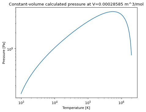
Through experience, it is observed that this behavior is only shown for some sets of critical constants. It was found that if the expression for $\frac{\partial P}{\partial T}_{V}$ is set to zero, an analytical expression can be determined for exactly what that maximum pressure is. Some EOSs implement this function as P_max_at_V; those that don’t, and fluids where there is no maximum pressure, will have that method but it will return None.

Debug Plots to Understand EOSs

The GCEOS.volume_errors method shows the relative error in the volume solution. mpmath is requried for this functionality. It is not likely there is an error here but many problems have been found in the past.

(Source code, png, hires.png, pdf)

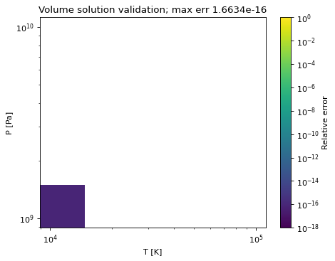
The GCEOS.PT_surface_special method shows some of the special curves of the EOS.

(Source code, png, hires.png, pdf)

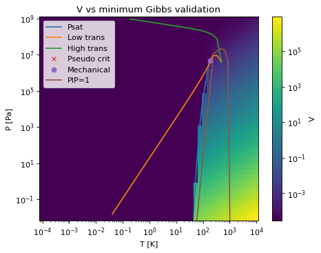
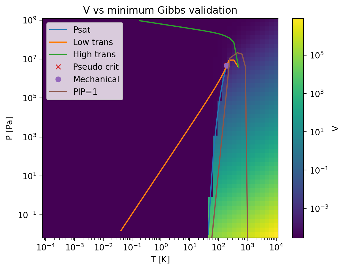
The GCEOS.a_alpha_plot method shows the alpha function curve. The following sample shows the SRK’s default alpha function for methane.

(Source code, png, hires.png, pdf)

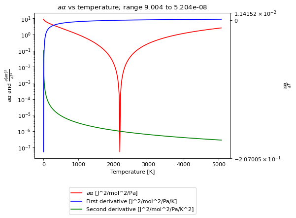
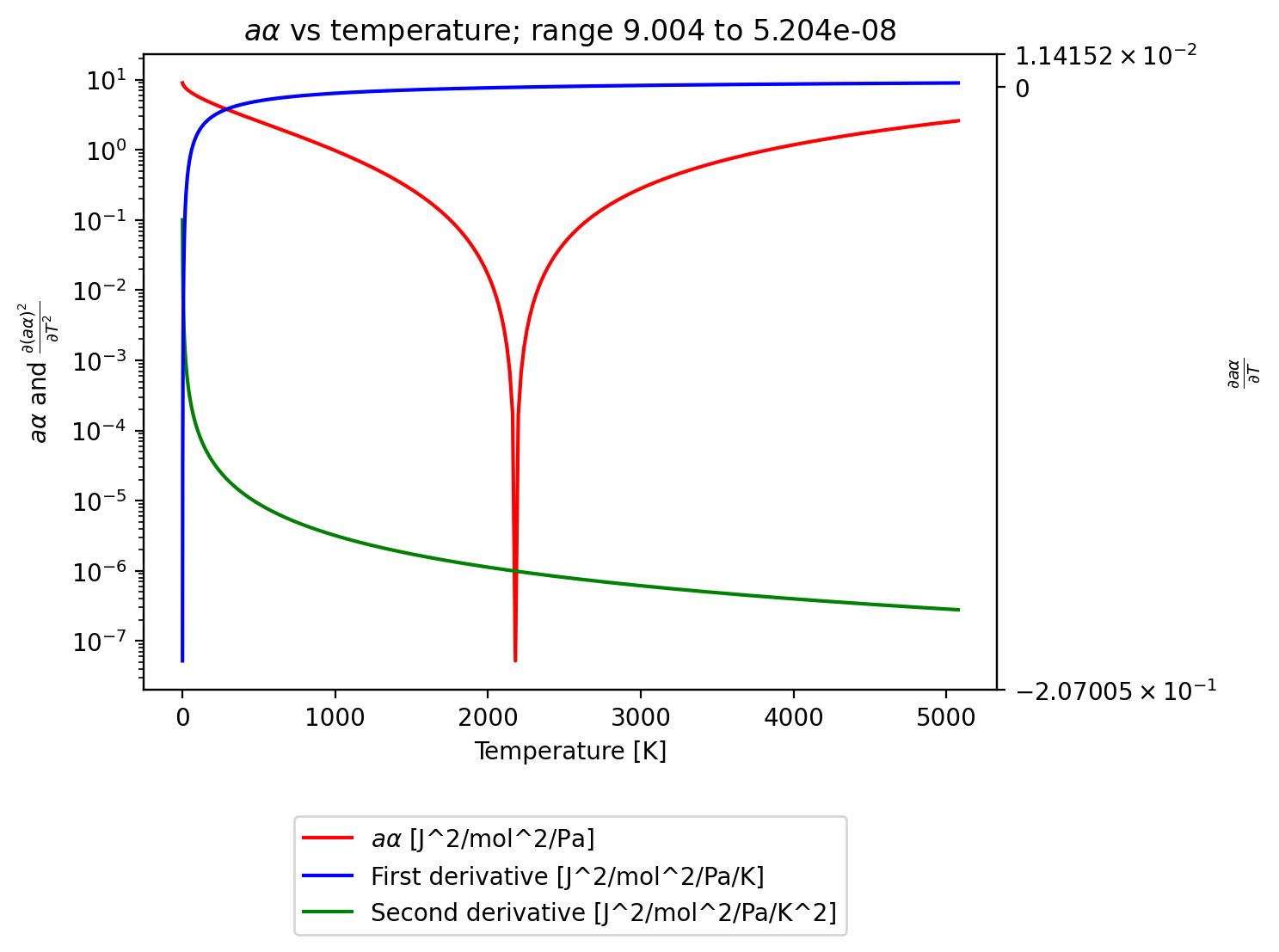
If this doesn’t look healthy, that is because it is not. There are strict thermodynamic consistency requirements that we know of today:

• The alpha function must be positive and continuous

• The first derivative must be negative and continuous

• The second derivative must be positive and continuous

• The third derivative must be negative

The first criterial and second criteria fail here.

There are two methods to review the saturation properties solution. The more general way is to review saturation properties as a plot:

(Source code, png, hires.png, pdf)

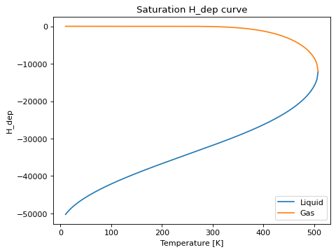
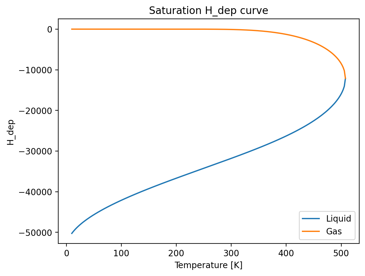
(Source code, png, hires.png, pdf)

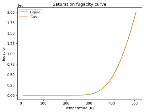
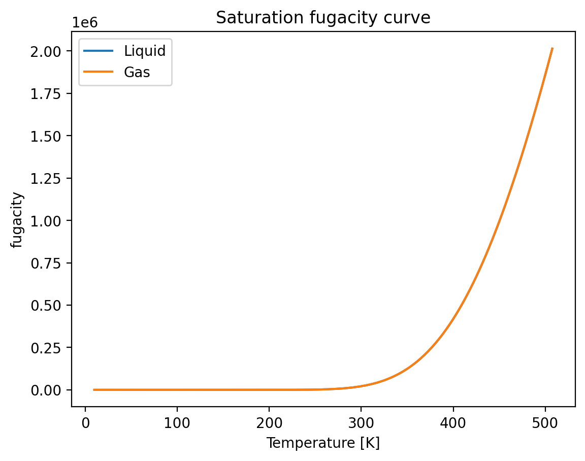
The second plot is more detailed, and is focused on the direct calculation of vapor pressure without using an iterative solution. It shows the relative error of the fit, which normally way below where it would present any issue - only 10-100x more error than it is possible to get with floating point numbers at all.

(Source code, png, hires.png, pdf)
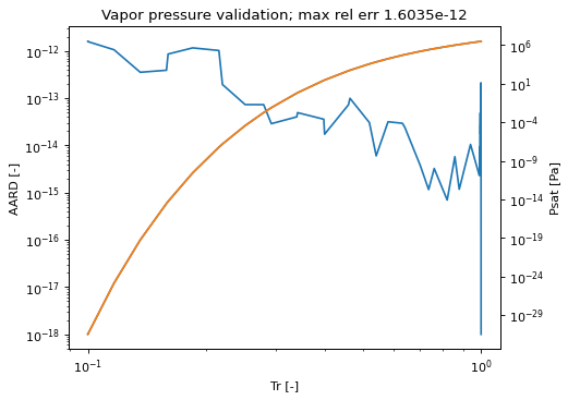
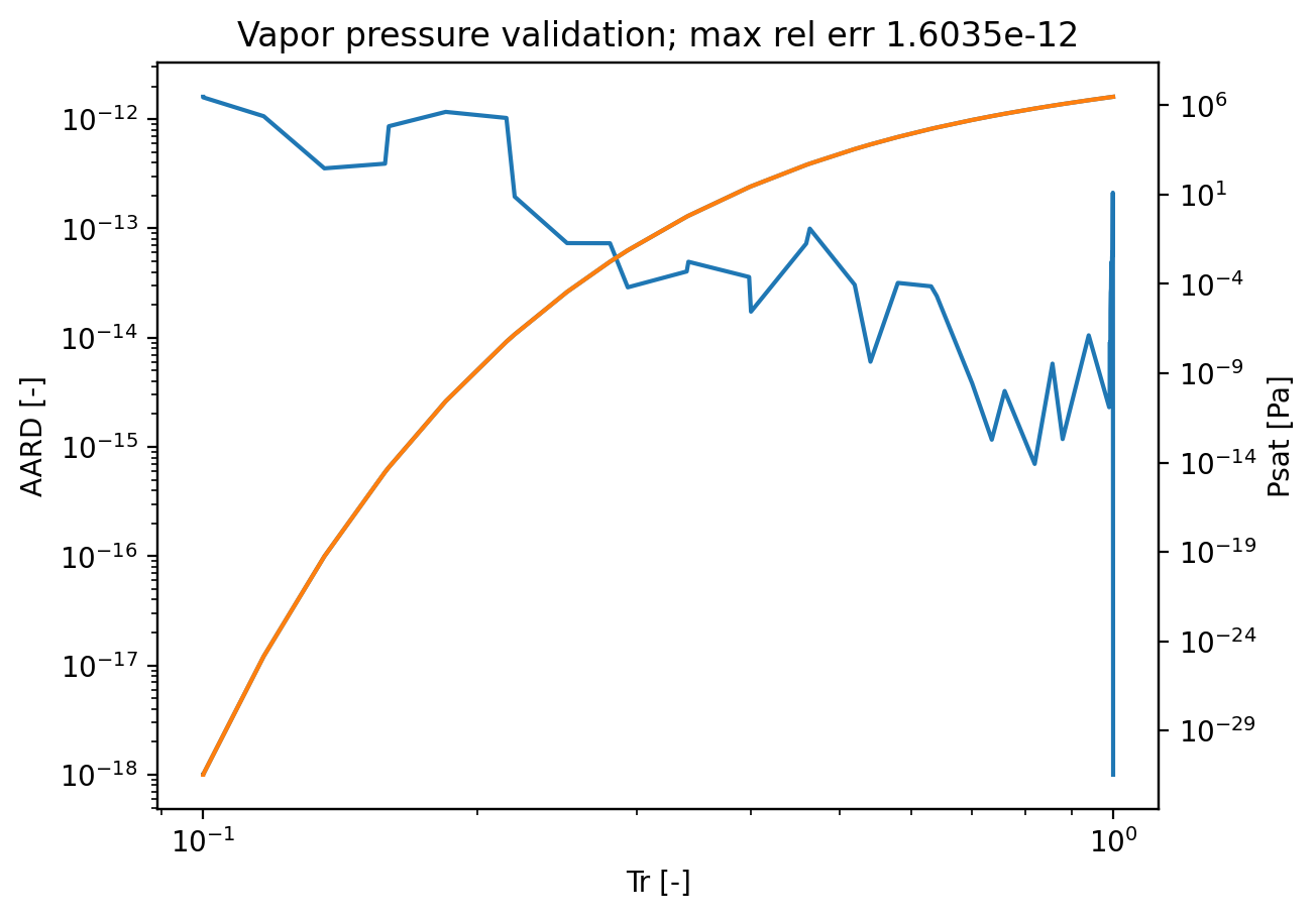