Cubic Equations of State Volume Solvers (thermo.eos_volume)

Some of the methods implemented here are numerical while others are analytical.

The cubic EOS can be rearranged into the following polynomial form:

$$0 = Z^3 + (\delta' - B' - 1)Z^2 + [\theta' + \epsilon' - \delta(B'+1)]Z - [\epsilon'(B'+1) + \theta'\eta']$$

$$B' = \frac{bP}{RT}$$

$$\delta' = \frac{\delta P}{RT}$$

$$\theta' = \frac{a\alpha P}{(RT)^2}$$

$$\epsilon' = \epsilon\left(\frac{P}{RT}\right)^2$$

The range of pressures, temperatures, and $a \alpha$ values is so large that almost all analytical solutions produce huge errors in some conditions. Because the EOS volume cannot be under b, this often results in a root being ignored where there should have been a liquid-like root detected.

A number of plots showing the relative error in volume calculation are shown below to demonstrate how different methods work.

Analytical Solvers

thermo.eos_volume.volume_solutions_Cardano(T, P, b, delta, epsilon, a_alpha)

Calculate the molar volume solutions to a cubic equation of state using Cardano’s formula, and a few tweaks to improve numerical precision. This solution is quite fast in general although it involves powers or trigonometric functions. However, it has numerical issues at many seemingly random areas in the low pressure region.

Parameters

Tfloat

Temperature, [K]

Pfloat

Pressure, [Pa]

bfloat

Coefficient calculated by EOS-specific method, [m^3/mol]

deltafloat

Coefficient calculated by EOS-specific method, [m^3/mol]

epsilonfloat

Coefficient calculated by EOS-specific method, [m^6/mol^2]

a_alphafloat

Coefficient calculated by EOS-specific method, [J^2/mol^2/Pa]

Returns

Vslist[float]

Three possible molar volumes, [m^3/mol]

Notes

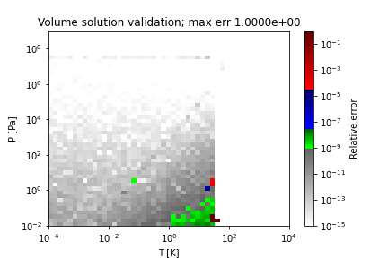
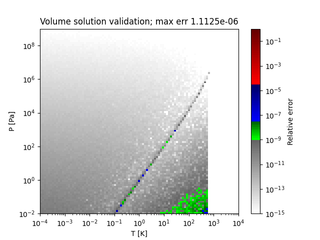
Two sample regions where this method does not obtain the correct solution (PR EOS for hydrogen) are as follows:

References

1

Reid, Robert C.; Prausnitz, John M.; Poling, Bruce E. Properties of Gases and Liquids. McGraw-Hill Companies, 1987.

thermo.eos_volume.volume_solutions_fast(T, P, b, delta, epsilon, a_alpha)

Solution of this form of the cubic EOS in terms of volumes. Returns three values, all with some complex part. This is believed to be the fastest analytical formula, and while it does not suffer from the same errors as Cardano’s formula, it has plenty of its own numerical issues.

Parameters

Tfloat

Temperature, [K]

Pfloat

Pressure, [Pa]

bfloat

Coefficient calculated by EOS-specific method, [m^3/mol]

deltafloat

Coefficient calculated by EOS-specific method, [m^3/mol]

epsilonfloat

Coefficient calculated by EOS-specific method, [m^6/mol^2]

a_alphafloat

Coefficient calculated by EOS-specific method, [J^2/mol^2/Pa]

Returns

Vstuple[complex]

Three possible molar volumes, [m^3/mol]

Notes

Using explicit formulas, as can be derived in the following example, is faster than most numeric root finding techniques, and finds all values explicitly. It takes several seconds.

>>> from sympy import *
>>> P, T, V, R, b, a, delta, epsilon, alpha = symbols('P, T, V, R, b, a, delta, epsilon, alpha')
>>> Tc, Pc, omega = symbols('Tc, Pc, omega')
>>> CUBIC = R*T/(V-b) - a*alpha/(V*V + delta*V + epsilon) - P
>>> #solve(CUBIC, V)

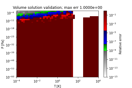
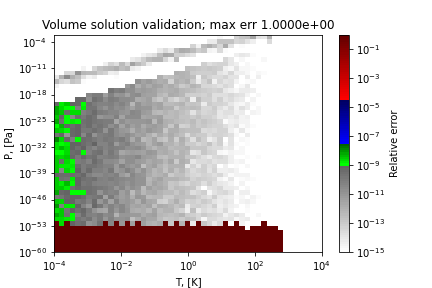
A sample region where this method does not obtain the correct solution (PR EOS for methanol) is as follows:

References

1

Zhi, Yun, and Huen Lee. “Fallibility of Analytic Roots of Cubic Equations of State in Low Temperature Region.” Fluid Phase Equilibria 201, no. 2 (September 30, 2002): 287-94. https://doi.org/10.1016/S0378-3812(02)00072-9.

thermo.eos_volume.volume_solutions_a1(T, P, b, delta, epsilon, a_alpha)

Solution of this form of the cubic EOS in terms of volumes. Returns three values, all with some complex part. This uses an analytical solution for the cubic equation with the leading coefficient set to 1 as in the EOS case; and the analytical solution is the one recommended by Mathematica.

Parameters

Tfloat

Temperature, [K]

Pfloat

Pressure, [Pa]

bfloat

Coefficient calculated by EOS-specific method, [m^3/mol]

deltafloat

Coefficient calculated by EOS-specific method, [m^3/mol]

epsilonfloat

Coefficient calculated by EOS-specific method, [m^6/mol^2]

a_alphafloat

Coefficient calculated by EOS-specific method, [J^2/mol^2/Pa]

Returns

Vstuple[complex]

Three possible molar volumes, [m^3/mol]

Notes

A sample region where this method does not obtain the correct solution (PR EOS for methanol) is as follows:

Examples

Numerical precision is always challenging and has edge cases. The following results all havev imaginary components, but depending on the math library used by the compiler even the first complex digit may not match!

>>> volume_solutions_a1(8837.07874361444, 216556124.0631852, 0.0003990176625589891, 0.0010590390565805598, -1.5069972655436541e-07, 7.20417995032918e-15) 
((0.000738308-7.5337e-20j), (-0.001186094-6.52444e-20j), (0.000127055+6.52444e-20j))

thermo.eos_volume.volume_solutions_a2(T, P, b, delta, epsilon, a_alpha)

Solution of this form of the cubic EOS in terms of volumes. Returns three values, all with some complex part. This uses an analytical solution for the cubic equation with the leading coefficient set to 1 as in the EOS case; and the analytical solution is the one recommended by Maple.

Parameters

Tfloat

Temperature, [K]

Pfloat

Pressure, [Pa]

bfloat

Coefficient calculated by EOS-specific method, [m^3/mol]

deltafloat

Coefficient calculated by EOS-specific method, [m^3/mol]

epsilonfloat

Coefficient calculated by EOS-specific method, [m^6/mol^2]

a_alphafloat

Coefficient calculated by EOS-specific method, [J^2/mol^2/Pa]

Returns

Vstuple[complex]

Three possible molar volumes, [m^3/mol]

Notes

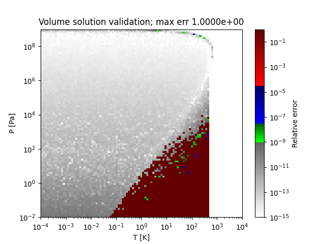
A sample region where this method does not obtain the correct solution (SRK EOS for decane) is as follows:

thermo.eos_volume.volume_solutions_numpy(T, P, b, delta, epsilon, a_alpha)

Calculate the molar volume solutions to a cubic equation of state using NumPy’s roots function, which is a power series iterative matrix solution that is very stable but does not have full precision in some cases.

Parameters

Tfloat

Temperature, [K]

Pfloat

Pressure, [Pa]

bfloat

Coefficient calculated by EOS-specific method, [m^3/mol]

deltafloat

Coefficient calculated by EOS-specific method, [m^3/mol]

epsilonfloat

Coefficient calculated by EOS-specific method, [m^6/mol^2]

a_alphafloat

Coefficient calculated by EOS-specific method, [J^2/mol^2/Pa]

Returns

Vslist[float]

Three possible molar volumes, [m^3/mol]

Notes

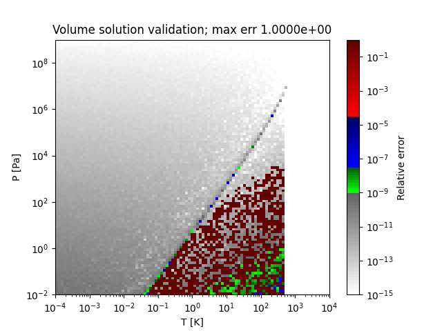
A sample region where this method does not obtain the correct solution (SRK EOS for ethane) is as follows:

References

1

Reid, Robert C.; Prausnitz, John M.; Poling, Bruce E. Properties of Gases and Liquids. McGraw-Hill Companies, 1987.

thermo.eos_volume.volume_solutions_ideal(T, P, b=0.0, delta=0.0, epsilon=0.0, a_alpha=0.0)

Calculate the ideal-gas molar volume in a format compatible with the other cubic EOS solvers. The ideal gas volume is the first element; and the secodn and third elements are zero. This is implemented to allow the ideal-gas model to be compatible with the cubic models, whose equations do not work with parameters of zero.

Parameters

Tfloat

Temperature, [K]

Pfloat

Pressure, [Pa]

bfloat, optional

Coefficient calculated by EOS-specific method, [m^3/mol]

deltafloat, optional

Coefficient calculated by EOS-specific method, [m^3/mol]

epsilonfloat, optional

Coefficient calculated by EOS-specific method, [m^6/mol^2]

a_alphafloat, optional

Coefficient calculated by EOS-specific method, [J^2/mol^2/Pa]

Returns

Vslist[float]

Three possible molar volumes, [m^3/mol]

Examples

>>> volume_solutions_ideal(T=300, P=1e7)
(0.0002494338785445972, 0.0, 0.0)

Numerical Solvers

thermo.eos_volume.volume_solutions_halley(T, P, b, delta, epsilon, a_alpha)

Halley’s method based solver for cubic EOS volumes based on the idea of initializing from a single liquid-like guess which is solved precisely, deflating the cubic analytically, solving the quadratic equation for the next two volumes, and then performing two halley steps on each of them to obtain the final solutions. This method does not calculate imaginary roots - they are set to zero on detection. This method has been rigorously tested over a wide range of conditions.

The method uses the standard combination of bisection to provide high and low boundaries as well, to keep the iteration always moving forward.

Parameters

Tfloat

Temperature, [K]

Pfloat

Pressure, [Pa]

bfloat

Coefficient calculated by EOS-specific method, [m^3/mol]

deltafloat

Coefficient calculated by EOS-specific method, [m^3/mol]

epsilonfloat

Coefficient calculated by EOS-specific method, [m^6/mol^2]

a_alphafloat

Coefficient calculated by EOS-specific method, [J^2/mol^2/Pa]

Returns

Vstuple[float]

Three possible molar volumes, [m^3/mol]

Notes

A sample region where this method works perfectly is shown below:

thermo.eos_volume.volume_solutions_NR(T, P, b, delta, epsilon, a_alpha, tries=0)

Newton-Raphson based solver for cubic EOS volumes based on the idea of initializing from an analytical solver. This algorithm can only be described as a monstrous mess. It is fairly fast for most cases, but about 3x slower than volume_solutions_halley. In the worst case this will fall back to mpmath.

Parameters

Tfloat

Temperature, [K]

Pfloat

Pressure, [Pa]

bfloat

Coefficient calculated by EOS-specific method, [m^3/mol]

deltafloat

Coefficient calculated by EOS-specific method, [m^3/mol]

epsilonfloat

Coefficient calculated by EOS-specific method, [m^6/mol^2]

a_alphafloat

Coefficient calculated by EOS-specific method, [J^2/mol^2/Pa]

triesint, optional

Internal parameter as this function will call itself if it needs to; number of previous solve attempts, [-]

Returns

Vstuple[complex]

Three possible molar volumes, [m^3/mol]

Notes

Sample regions where this method works perfectly are shown below:

thermo.eos_volume.volume_solutions_NR_low_P(T, P, b, delta, epsilon, a_alpha)

Newton-Raphson based solver for cubic EOS volumes designed specifically for the low-pressure regime. Seeks only two possible solutions - an ideal gas like one, and one near the eos covolume b - as the initializations are R*T/P and b*1.000001 .

Parameters

Tfloat

Temperature, [K]

Pfloat

Pressure, [Pa]

bfloat

Coefficient calculated by EOS-specific method, [m^3/mol]

deltafloat

Coefficient calculated by EOS-specific method, [m^3/mol]

epsilonfloat

Coefficient calculated by EOS-specific method, [m^6/mol^2]

a_alphafloat

Coefficient calculated by EOS-specific method, [J^2/mol^2/Pa]

triesint, optional

Internal parameter as this function will call itself if it needs to; number of previous solve attempts, [-]

Returns

Vstuple[complex]

Three possible molar volumes (third one is hardcoded to 1j), [m^3/mol]

Notes

The algorithm is NR, with some checks that will switch the solver to brenth some of the time.

Higher-Precision Solvers

thermo.eos_volume.volume_solutions_mpmath(T, P, b, delta, epsilon, a_alpha, dps=50)

Solution of this form of the cubic EOS in terms of volumes, using the mpmath arbitrary precision library. The number of decimal places returned is controlled by the dps parameter.

This function is the reference implementation which provides exactly correct solutions; other algorithms are compared against this one.

Parameters

Tfloat

Temperature, [K]

Pfloat

Pressure, [Pa]

bfloat

Coefficient calculated by EOS-specific method, [m^3/mol]

deltafloat

Coefficient calculated by EOS-specific method, [m^3/mol]

epsilonfloat

Coefficient calculated by EOS-specific method, [m^6/mol^2]

a_alphafloat

Coefficient calculated by EOS-specific method, [J^2/mol^2/Pa]

dpsint

Number of decimal places in the result by mpmath, [-]

Returns

Vstuple[complex]

Three possible molar volumes, [m^3/mol]

Notes

Although mpmath has a cubic solver, it has been found to fail to solve in some cases. Accordingly, the algorithm is as follows:

Working precision is dps plus 40 digits; and if P < 1e-10 Pa, it is dps plus 400 digits. The input parameters are converted exactly to mpf objects on input.

polyroots from mpmath is used with maxsteps=2000, and extra precision of 15 digits. If the solution does not converge, 20 extra digits are added up to 8 times. If no solution is found, mpmath’s findroot is called on the pressure error function using three initial guesses from another solver.

Needless to say, this function is quite slow.

References

1

Johansson, Fredrik. Mpmath: A Python Library for Arbitrary-Precision Floating-Point Arithmetic, 2010.

Examples

Test case which presented issues for PR EOS (three roots were not being returned):

>>> volume_solutions_mpmath(0.01, 1e-05, 2.5405184201558786e-05, 5.081036840311757e-05, -6.454233843151321e-10, 0.3872747173781095)
(mpf('0.0000254054613415548712260258773060137'), mpf('4.66038025602155259976574392093252'), mpf('8309.80218708657190094424659859346'))

thermo.eos_volume.volume_solutions_mpmath_float(T, P, b, delta, epsilon, a_alpha)

Simple wrapper around volume_solutions_mpmath which uses the default parameters and returns the values as floats.

Parameters

Tfloat

Temperature, [K]

Pfloat

Pressure, [Pa]

bfloat

Coefficient calculated by EOS-specific method, [m^3/mol]

deltafloat

Coefficient calculated by EOS-specific method, [m^3/mol]

epsilonfloat

Coefficient calculated by EOS-specific method, [m^6/mol^2]

a_alphafloat

Coefficient calculated by EOS-specific method, [J^2/mol^2/Pa]

dpsint

Number of decimal places in the result by mpmath, [-]

Returns

Vstuple[complex]

Three possible molar volumes, [m^3/mol]

Examples

Test case which presented issues for PR EOS (three roots were not being returned):

>>> volume_solutions_mpmath_float(0.01, 1e-05, 2.5405184201558786e-05, 5.081036840311757e-05, -6.454233843151321e-10, 0.3872747173781095)
((2.540546134155487e-05+0j), (4.660380256021552+0j), (8309.802187086572+0j))

thermo.eos_volume.volume_solutions_sympy(T, P, b, delta, epsilon, a_alpha)

Solution of this form of the cubic EOS in terms of volumes, using the sympy mathematical library with real numbers.

This function is generally slow, and somehow still has more than desired error in the real and complex result.

$$V_0 = - \frac{- \frac{3 \left(- P b \delta + P \epsilon - R T \delta + a \alpha\right)}{P} + \frac{\left(- P b + P \delta - R T\right)^{2}} {P^{2}}}{3 \sqrt[3]{\frac{\sqrt{- 4 \left(- \frac{3 \left(- P b \delta + P \epsilon - R T \delta + a \alpha\right)}{P} + \frac{\left(- P b + P \delta - R T\right)^{2}}{P^{2}}\right)^{3} + \left(\frac{27 \left( - P b \epsilon - R T \epsilon - a \alpha b\right)}{P} - \frac{9 \left(- P b + P \delta - R T\right) \left(- P b \delta + P \epsilon - R T \delta + a \alpha\right)}{P^{2}} + \frac{2 \left(- P b + P \delta - R T\right)^{3}}{P^{3}}\right)^{2}}}{2} + \frac{27 \left(- P b \epsilon - R T \epsilon - a \alpha b\right)}{2 P} - \frac{9 \left(- P b + P \delta - R T\right) \left(- P b \delta + P \epsilon - R T \delta + a \alpha\right)}{2 P^{2}} + \frac{\left(- P b + P \delta - R T\right)^{3}} {P^{3}}}} - \frac{\sqrt[3]{\frac{\sqrt{- 4 \left(- \frac{3 \left(- P b \delta + P \epsilon - R T \delta + a \alpha\right)}{P} + \frac{\left(- P b + P \delta - R T\right)^{2}}{P^{2}}\right)^{3} + \left(\frac{27 \left( - P b \epsilon - R T \epsilon - a \alpha b\right)}{P} - \frac{9 \left( - P b + P \delta - R T\right) \left(- P b \delta + P \epsilon - R T \delta + a \alpha\right)}{P^{2}} + \frac{2 \left(- P b + P \delta - R T\right)^{3}}{P^{3}}\right)^{2}}}{2} + \frac{27 \left(- P b \epsilon - R T \epsilon - a \alpha b\right)}{2 P} - \frac{9 \left(- P b + P \delta - R T\right) \left(- P b \delta + P \epsilon - R T \delta + a \alpha\right)}{2 P^{2}} + \frac{\left(- P b + P \delta - R T \right)^{3}}{P^{3}}}}{3} - \frac{- P b + P \delta - R T}{3 P}$$

$$V_1 = - \frac{- \frac{3 \left(- P b \delta + P \epsilon - R T \delta + a \alpha\right)}{P} + \frac{\left(- P b + P \delta - R T\right)^{2}} {P^{2}}}{3 \left(- \frac{1}{2} - \frac{\sqrt{3} i}{2}\right) \sqrt[3] {\frac{\sqrt{- 4 \left(- \frac{3 \left(- P b \delta + P \epsilon - R T \delta + a \alpha\right)}{P} + \frac{\left(- P b + P \delta - R T \right)^{2}}{P^{2}}\right)^{3} + \left(\frac{27 \left(- P b \epsilon - R T \epsilon - a \alpha b\right)}{P} - \frac{9 \left(- P b + P \delta - R T\right) \left(- P b \delta + P \epsilon - R T \delta + a \alpha\right)}{P^{2}} + \frac{2 \left(- P b + P \delta - R T \right)^{3}}{P^{3}}\right)^{2}}}{2} + \frac{27 \left(- P b \epsilon - R T \epsilon - a \alpha b\right)}{2 P} - \frac{9 \left(- P b + P \delta - R T\right) \left(- P b \delta + P \epsilon - R T \delta + a \alpha\right)}{2 P^{2}} + \frac{\left(- P b + P \delta - R T \right)^{3}}{P^{3}}}} - \frac{\left(- \frac{1}{2} - \frac{\sqrt{3} i} {2}\right) \sqrt[3]{\frac{\sqrt{- 4 \left(- \frac{3 \left(- P b \delta + P \epsilon - R T \delta + a \alpha\right)}{P} + \frac{\left(- P b + P \delta - R T\right)^{2}}{P^{2}}\right)^{3} + \left(\frac{27 \left( - P b \epsilon - R T \epsilon - a \alpha b\right)}{P} - \frac{9 \left( - P b + P \delta - R T\right) \left(- P b \delta + P \epsilon - R T \delta + a \alpha\right)}{P^{2}} + \frac{2 \left(- P b + P \delta - R T\right)^{3}}{P^{3}}\right)^{2}}}{2} + \frac{27 \left(- P b \epsilon - R T \epsilon - a \alpha b\right)}{2 P} - \frac{9 \left(- P b + P \delta - R T\right) \left(- P b \delta + P \epsilon - R T \delta + a \alpha\right)}{2 P^{2}} + \frac{\left(- P b + P \delta - R T \right)^{3}}{P^{3}}}}{3} - \frac{- P b + P \delta - R T}{3 P}$$

$$V_2 = - \frac{- \frac{3 \left(- P b \delta + P \epsilon - R T \delta + a \alpha\right)}{P} + \frac{\left(- P b + P \delta - R T\right)^{2}} {P^{2}}}{3 \left(- \frac{1}{2} + \frac{\sqrt{3} i}{2}\right) \sqrt[3] {\frac{\sqrt{- 4 \left(- \frac{3 \left(- P b \delta + P \epsilon - R T \delta + a \alpha\right)}{P} + \frac{\left(- P b + P \delta - R T \right)^{2}}{P^{2}}\right)^{3} + \left(\frac{27 \left(- P b \epsilon - R T \epsilon - a \alpha b\right)}{P} - \frac{9 \left(- P b + P \delta - R T\right) \left(- P b \delta + P \epsilon - R T \delta + a \alpha \right)}{P^{2}} + \frac{2 \left(- P b + P \delta - R T\right)^{3}} {P^{3}}\right)^{2}}}{2} + \frac{27 \left(- P b \epsilon - R T \epsilon - a \alpha b\right)}{2 P} - \frac{9 \left(- P b + P \delta - R T\right) \left(- P b \delta + P \epsilon - R T \delta + a \alpha\right)}{2 P^{2}} + \frac{\left(- P b + P \delta - R T\right)^{3}}{P^{3}}}} - \frac{\left( - \frac{1}{2} + \frac{\sqrt{3} i}{2}\right) \sqrt[3]{\frac{\sqrt{- 4 \left(- \frac{3 \left(- P b \delta + P \epsilon - R T \delta + a \alpha \right)}{P} + \frac{\left(- P b + P \delta - R T\right)^{2}}{P^{2}} \right)^{3} + \left(\frac{27 \left(- P b \epsilon - R T \epsilon - a \alpha b\right)}{P} - \frac{9 \left(- P b + P \delta - R T\right) \left(- P b \delta + P \epsilon - R T \delta + a \alpha\right)}{P^{2}} + \frac{2 \left(- P b + P \delta - R T\right)^{3}}{P^{3}}\right)^{2}}} {2} + \frac{27 \left(- P b \epsilon - R T \epsilon - a \alpha b\right)} {2 P} - \frac{9 \left(- P b + P \delta - R T\right) \left(- P b \delta + P \epsilon - R T \delta + a \alpha\right)}{2 P^{2}} + \frac{\left( - P b + P \delta - R T\right)^{3}}{P^{3}}}}{3} - \frac{- P b + P \delta - R T}{3 P}$$

Parameters

Tfloat

Temperature, [K]

Pfloat

Pressure, [Pa]

bfloat

Coefficient calculated by EOS-specific method, [m^3/mol]

deltafloat

Coefficient calculated by EOS-specific method, [m^3/mol]

epsilonfloat

Coefficient calculated by EOS-specific method, [m^6/mol^2]

a_alphafloat

Coefficient calculated by EOS-specific method, [J^2/mol^2/Pa]

Returns

Vstuple[sympy.Rational]

Three possible molar volumes, [m^3/mol]

Notes

The solution can be derived as follows:

>>> from sympy import * 
>>> P, T, V, R, b, delta, epsilon = symbols('P, T, V, R, b, delta, epsilon') 
>>> a_alpha = Symbol(r'a \alpha') 
>>> CUBIC = R*T/(V-b) - a_alpha/(V*V + delta*V + epsilon) - P 
>>> V_slns = solve(CUBIC, V) 

References

1

Meurer, Aaron, Christopher P. Smith, Mateusz Paprocki, Ondřej Čertík, Sergey B. Kirpichev, Matthew Rocklin, AMiT Kumar, Sergiu Ivanov, Jason K. Moore, and Sartaj Singh. “SymPy: Symbolic Computing in Python.” PeerJ Computer Science 3 (2017): e103.

Examples

>>> Vs = volume_solutions_sympy(0.01, 1e-05, 2.5405184201558786e-05, 5.081036840311757e-05, -6.454233843151321e-10, 0.3872747173781095) 
>>> [complex(v) for v in Vs] 
[(2.540546e-05+2.402202278e-12j), (4.660380256-2.40354958e-12j), (8309.80218+1.348096981e-15j)]