Introduction to Property Objects

For every chemical property, there are lots and lots of methods. The methods can be grouped by which phase they apply to, although some methods are valid for both liquids and gases.

Properties calculations be separated into three categories:

• Properties of chemicals that depend on temperature. Some properties have weak dependence on pressure, like surface tension, and others have no dependence on pressure like vapor pressure by definition.

• Properties of chemicals that depend on temperature and pressure. Some properties have weak dependence on pressure like thermal conductivity, while other properties depend on pressure fundamentally, like gas volume.

• Properties of mixtures, that depend on temperature and pressure and composition. Some properties like gas mixture heat capacity require the pressure as an input but do not use it.

These properties are implemented in an object oriented way, with the actual functional algorithms themselves having been separated out into the chemicals library. The goal of these objects is to make it easy to experiment with different methods.

The base classes for the three respective types of properties are:

• TDependentProperty

• TPDependentProperty

• MixtureProperty

The specific classes for the three respective types of properties are:

• HeatCapacityGas, HeatCapacityLiquid, HeatCapacitySolid, VolumeSolid, VaporPressure, SublimationPressure, EnthalpyVaporization, EnthalpySublimation, Permittivity, SurfaceTension.

• VolumeGas, VolumeLiquid, ViscosityGas, ViscosityLiquid, ThermalConductivityGas, ThermalConductivityLiquid

• HeatCapacityGasMixture, HeatCapacityLiquidMixture, HeatCapacitySolidMixture, VolumeGasMixture, VolumeLiquidMixture, VolumeSolidMixture, ViscosityLiquidMixture, ViscosityGasMixture, ThermalConductivityLiquidMixture, ThermalConductivityGasMixture, SurfaceTensionMixture

Temperature Dependent Properties

The following examples introduce how to use some of the methods of the TDependentProperty objects. The API documentation for TDependentProperty as well as each specific property such as VaporPressure should be consulted for full details.

Creating Objects

All arguments and information the property object requires must be provided in the constructor of the object. If a piece of information is not provided, whichever methods require it will not be available for that object.

>>> from thermo import VaporPressure, HeatCapacityGas
>>> ethanol_psat = VaporPressure(Tb=351.39, Tc=514.0, Pc=6137000.0, omega=0.635, CASRN='64-17-5')

Various data files will be searched to see if information such as Antoine coefficients is available for the compound during the initialization. This behavior can be avoided by setting the optional load_data argument to False. Loading data requires pandas, uses more RAM, and is a once-per-process procedure that takes 20-1000 ms per property. For some applications it may be advantageous to provide your own data instead of using the provided data files.

>>> useless_psat = VaporPressure(CASRN='64-17-5', load_data=False)

Temperature-dependent Methods

As many methods may be available, a single method is always selected automatically during initialization. This method can be inspected with the method property; if no methods are available, method will be None. method is also a valid parameter when constructing the object, but if the method specified is not available an exception will be raised.

>>> ethanol_psat.method, useless_psat.method
('HEOS_FIT', None)

All available methods can be found by inspecting the all_methods attribute:

>>> ethanol_psat.all_methods 
{'HEOS_FIT', 'WAGNER_POLING', 'WAGNER_MCGARRY', 'LEE_KESLER_PSAT', 'ANTOINE_WEBBOOK', 'AMBROSE_WALTON', 'DIPPR_PERRY_8E', 'VDI_PPDS', 'ANTOINE_POLING', 'COOLPROP', 'EDALAT', 'VDI_TABULAR', 'SANJARI', 'BOILING_CRITICAL'}

Changing the method is as easy as setting a new value to the attribute:

>>> ethanol_psat.method = 'ANTOINE_POLING'
>>> ethanol_psat.method
'ANTOINE_POLING'
>>> ethanol_psat.method = 'WAGNER_MCGARRY'

Calculating Properties

Calculation of the property at a specific temperature is as easy as calling the object which triggers the __call__ method:

>>> ethanol_psat(300.0)
8753.8160

This is actually a cached wrapper around the specific call, T_dependent_property:

>>> ethanol_psat.T_dependent_property(300.0)
8753.8160

The caching of __call__ is quite basic - the previously specified temperature is stored, and if the new T is the same as the previous T the previously calculated result is returned.

There is a lower-level interface for calculating properties with a specified method by name, calculate. T_dependent_property is a wrapper around calculate that includes validation of the result.

>>> ethanol_psat.calculate(T=300.0, method='WAGNER_MCGARRY')
8753.8160
>>> ethanol_psat.calculate(T=300.0, method='DIPPR_PERRY_8E')
8812.9812

Limits and Extrapolation

Each correlation is associated with temperature limits. These can be inspected as part of the T_limits attribute which is loaded on creation of the property object.

>>> ethanol_psat.T_limits 
{'WAGNER_MCGARRY': (293.0, 513.92), 'WAGNER_POLING': (159.05, 513.92), 'ANTOINE_POLING': (276.5, 369.54), 'DIPPR_PERRY_8E': (159.05, 514.0), 'COOLPROP': (159.1, 514.71), 'VDI_TABULAR': (300.0, 513.9), 'VDI_PPDS': (159.05, 513.9), 'BOILING_CRITICAL': (0.01, 514.0), 'LEE_KESLER_PSAT': (0.01, 514.0), 'AMBROSE_WALTON': (0.01, 514.0), 'SANJARI': (0.01, 514.0), 'EDALAT': (0.01, 514.0)}

Because there is often a need to obtain a property outside the range of the correlation, there are some extrapolation methods available; depending on the method these may be enabled by default. The full list of extrapolation methods can be see here.

For vapor pressure, there are actually two separate extrapolation techniques used, one for the low-pressure and thermodynamically reasonable region and another for extrapolating even past the critical point. This can be useful for obtaining initial estimates of phase equilibrium.

The low-pressure region uses $\log(P_{sat}) = A - B/T$, where the coefficients A and B are calculated from the low-temperature limit and its temperature derivative. The default high-temperature extrapolation is $P_{sat} = \exp\left(A + B/T + C\log(T)\right)$. The coefficients are also determined from the high-temperature limits and its first two temperature derivatives.

When extrapolation is turned on, it is used automatically if a property is requested out of range:

>>> ethanol_psat(100.0), ethanol_psat(1000)
(1.047582e-11, 1779196575.4962692)

The default extrapolation methods may be changed in the future, but can be manually specified also by changing the value of the extrapolation attribute. For example, if the linear extrapolation method is set, extrapolation will be linear instead of using those fit equations. Because not all properties are suitable for linear extrapolation, some methods have a default transform to make the property behave as linearly as possible. This is also used in tabular interpolation:

>>> ethanol_psat.extrapolation = 'linear'
>>> ethanol_psat(100.0), ethanol_psat(1000)
(1.0475e-11, 385182009.4)

The low-temperature linearly extrapolated value is actually the same as before, because it performs a 1/T transform and a log(P) transform on the output, which results in the fit being the same as the default equation for vapor pressure.

To better understand what methods are available, the valid_methods method checks all available correlations against their temperature limits.

>>> ethanol_psat.valid_methods(100)
['AMBROSE_WALTON', 'LEE_KESLER_PSAT', 'EDALAT', 'BOILING_CRITICAL', 'SANJARI']

If the temperature is not provided, all available methods are returned; the returned value favors the methods by the ranking defined in thermo, with the currently selected method as the first item.

>>> ethanol_psat.valid_methods() 
['WAGNER_MCGARRY', 'WAGNER_POLING', 'DIPPR_PERRY_8E', 'VDI_PPDS', 'COOLPROP', 'ANTOINE_POLING', 'VDI_TABULAR', 'AMBROSE_WALTON', 'LEE_KESLER_PSAT', 'EDALAT', 'BOILING_CRITICAL', 'SANJARI']

Plotting

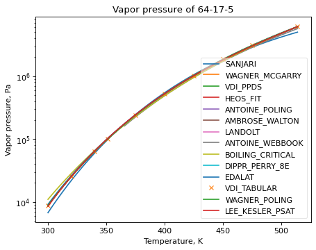
It is also possible to compare the correlations graphically with the method plot_T_dependent_property.

>>> ethanol_psat.plot_T_dependent_property(Tmin=300) 

(Source code, png, hires.png, pdf)

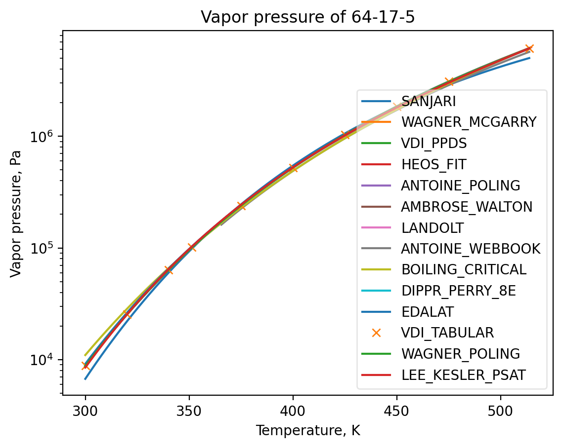
By default all methods are shown in the plot, but a smaller selection of methods can be specified. The following example compares 30 points in the temperature range 400 K to 500 K, with three of the best methods.

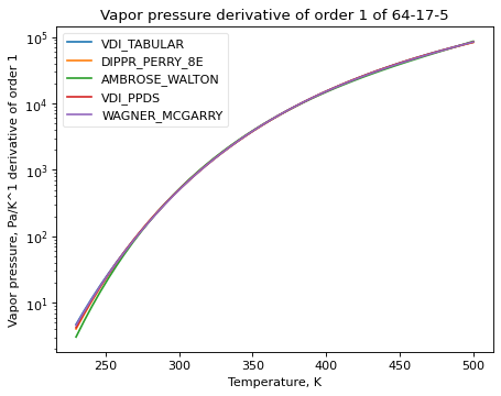
>>> ethanol_psat.plot_T_dependent_property(Tmin=400, Tmax=500, methods=['COOLPROP', 'WAGNER_MCGARRY', 'DIPPR_PERRY_8E'], pts=30) 

(Source code, png, hires.png, pdf)

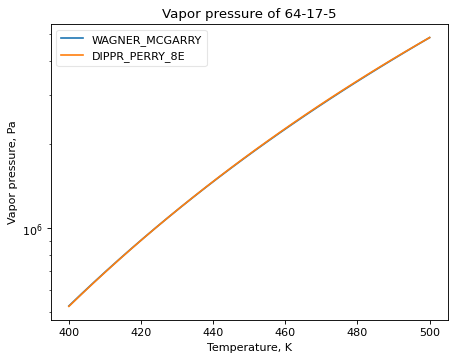
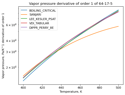
It is also possible to plot the nth derivative of the methods with the order parameter. The following plot shows the first derivative of vapor pressure of three estimation methods, a tabular source being interpolated, and ‘DIPPR_PERRY_8E’ as a reference method.

>>> ethanol_psat.plot_T_dependent_property(Tmin=400, Tmax=500, methods=['BOILING_CRITICAL', 'SANJARI', 'LEE_KESLER_PSAT', 'VDI_TABULAR', 'DIPPR_PERRY_8E'], pts=50, order=1) 

(Source code, png, hires.png, pdf)

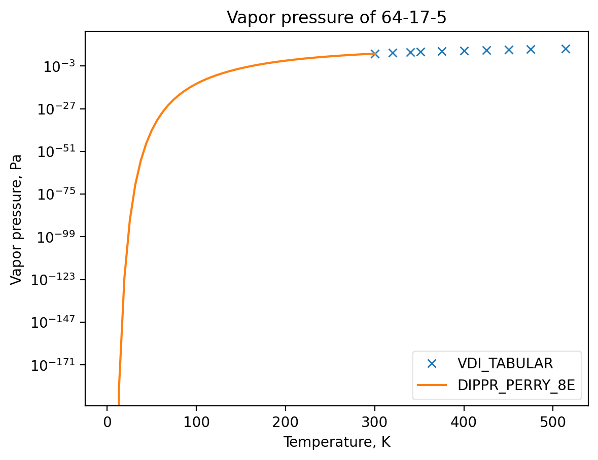
Plots show how the extrapolation methods work. By default plots do not show extrapolated values from methods, but this can be forced by setting only_valid to False. It is easy to see that extrapolation is designed to show the correct trend, but that individual methods will have very different extrapolations.

>>> ethanol_psat.plot_T_dependent_property(Tmin=1, Tmax=300, methods=['VDI_TABULAR', 'DIPPR_PERRY_8E', 'COOLPROP'], pts=50, only_valid=False) 

(Source code, png, hires.png, pdf)

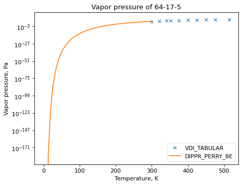
It may also be helpful to see the derivative with respect to temperature of methods. This can be done with the order keyword:

>>> ethanol_psat.plot_T_dependent_property(Tmin=1, Tmax=300, methods=['VDI_TABULAR', 'DIPPR_PERRY_8E', 'COOLPROP'], pts=50, only_valid=False, order=1) 

(Source code, png, hires.png, pdf)

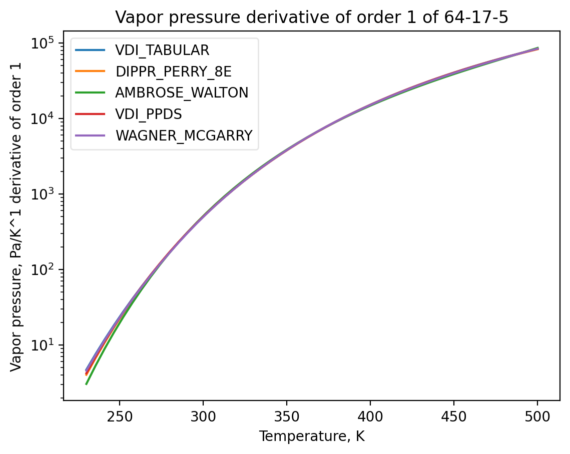
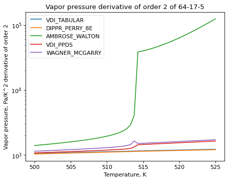
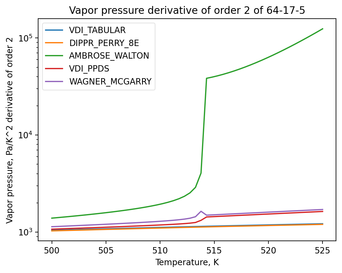
Higher order derivatives are also supported; most derivatives are numerically calculated, so there may be some noise. The derivative plot is particularly good at illustrating what happens at the critical point, when extrapolation takes over from the actual formulas.

>>> ethanol_psat.plot_T_dependent_property(Tmin=500, Tmax=525, methods=['VDI_TABULAR', 'DIPPR_PERRY_8E', 'AMBROSE_WALTON', 'VDI_PPDS', 'WAGNER_MCGARRY'], pts=50, only_valid=False, order=2) 

(Source code, png, hires.png, pdf)

Calculating Temperature From Properties

There is also functionality for reversing the calculation - finding out which temperature produces a specific property value. The method is solve_property. For vapor pressure, we can use this technique to find out the normal boiling point as follows:

>>> ethanol_psat.solve_property(101325)
351.43136

The experimentally reported value is 351.39 K.

Property Derivatives

Functionality for calculating the derivative of the property is also implemented as T_dependent_property_derivative :

>>> ethanol_psat.T_dependent_property_derivative(300)
498.882

The derivatives are numerical unless a special implementation has been added to the property’s calculate_derivative method.

Higher order derivatives are available as well with the order argument. All higher-order derivatives are numerical, and they tend to have reduced numerical precision due to floating point limitations.

>>> ethanol_psat.T_dependent_property_derivative(300.0, order=2)
24.74
>>> ethanol_psat.T_dependent_property_derivative(300.0, order=3)
2.75

Property Integrals

Functionality for integrating over a property is implemented as T_dependent_property_integral.

$$\text{integral} = \int_{T_1}^{T_2} \text{property} \; dT$$

When the property is heat capacity, this calculation represents a change in enthalpy:

$$\Delta H = \int_{T_1}^{T_2} C_p \; d T$$

>>> CH4_Cp = HeatCapacityGas(CASRN='74-82-8')
>>> CH4_Cp.method = 'POLING_POLY'
>>> CH4_Cp.T_dependent_property_integral(300, 500)
8158.64

Besides enthalpy, a commonly used integral is that of the property divided by T:

$$\text{integral} = \int_{T_1}^{T_2} \frac{\text{property}}{T} \; dT$$

When the property is heat capacity, this calculation represents a change in entropy:

$$\Delta S = \int_{T_1}^{T_2} \frac{C_p}{T} \; d T$$

This integral, property over T, is implemented as T_dependent_property_integral_over_T :

>>> CH4_Cp.T_dependent_property_integral_over_T(300, 500)
20.6088

Where speed has been important so far, these integrals have been implemented analytically in a property object’s calculate_integral and calculate_integral_over_T method; otherwise the integration is performed numerically.

Using Tabular Data

A common scenario is that there are no correlations available for a compound, and that estimation methods are not applicable. However, there may be a few experimental data points available in the literature. In this case, the data can be specified and used directly with the add_tabular_data method. Extrapolation can often show the correct trends for these properties from even a few data points.

In the example below, we take 5 data points on the vapor pressure of water from 300 K to 350 K, and use them to extrapolate and estimate the triple temperature and critical temperature (assuming we know the triple and critical pressures).

>>> from thermo import *
>>> import numpy as np
>>> w = VaporPressure(Tb=373.124, Tc=647.14, Pc=22048320.0, omega=0.344, CASRN='7732-18-5', extrapolation='AntoineAB')
>>> Ts = np.linspace(300, 350, 5).tolist()
>>> Ps = [3533.9, 7125., 13514., 24287., 41619.]
>>> w.add_tabular_data(Ts=Ts, properties=Ps)
>>> w.solve_property(610.707), w.solve_property(22048320)
(272.83, 617.9)

The experimental values are 273.15 K and 647.14 K.

Adding New Methods

While a great many property methods have been implemented, there is always the case where a new one must be added. To support that, the method add_method will add a user-specified method and switch the method selected to the newly added method.

As an example, we can compare the default vapor pressure formulation for n-hexane against a set of Antoine coefficients on the NIST WebBook.

>>> from chemicals import *
>>> from thermo import *
>>> obj = VaporPressure(CASRN= '110-54-3')
>>> obj(200)
20.39
>>> f = lambda T: Antoine(T=T, A=3.45604+5, B=1044.038, C=-53.893)
>>> obj.add_method(f=f, name='WebBook', Tmin=177.70, Tmax=264.93)
>>> obj.method
'WebBook'
>>> obj.extrapolation = 'AntoineAB'
>>> obj(200.0)
20.432

We can, again, extrapolate quite easily and estimate the triple temperature and critical temperature from these correlations (if we know the triple pressure and critical pressure).

>>> obj.solve_property(1.378), obj.solve_property(3025000.0)
(179.43, 508.04)

Optionally, some derivatives and integrals can be provided for new methods as well. This avoids having to compute derivatives or integrals numerically. SymPy may be helpful to find these analytical derivatives or integrals in many cases, as in the following example:

>>> from sympy import symbols, lambdify, diff
>>> T = symbols('T')
>>> A, B, C = 3.45604+5, 1044.038, -53.893
>>> expr = 10**(A - B/(T + C))
>>> f = lambdify(T, expr)
>>> f_der = lambdify(T, diff(expr, T))
>>> f_der2 = lambdify(T, diff(expr, T, 2))
>>> f_der3 = lambdify(T, diff(expr, T, 3))
>>> obj.add_method(f=f, f_der=f_der, f_der2=f_der2, f_der3=f_der3, name='WebBookSymPy', Tmin=177.70, Tmax=264.93)
>>> obj.method, obj(200), obj.T_dependent_property_derivative(200.0, order=2)
('WebBookSymPy', 20.43298036, 0.2276285)

Note that adding methods like this breaks the ability to export as json and the repr of the object is no longer complete.

Adding New Correlation Coefficient Methods

While adding entirely new methods is useful, it is more common to want to use different coefficients in an existing equation. A number of different equations are recognized, and accept/require the parameters as per their function name in e.g. chemicals.vapor_pressure.Antoine. More than one set of coefficients can be added for each model. After adding a new correlation the method is set to that method.

>>> obj = VaporPressure()
>>> obj.add_correlation(name='WebBook', model='Antoine', Tmin=177.70, Tmax=264.93,  A=3.45604+5, B=1044.038, C=-53.893)
>>> obj(200)
20.43298036711

It is also possible to specify the parameters in the constructor of the object as well:

>>> obj = VaporPressure(Antoine_parameters={'WebBook': {'A': 8.45604, 'B': 1044.038, 'C': -53.893, 'Tmin': 177.7, 'Tmax': 264.93}})
>>> obj(200)
20.43298036711

More than one set of parameters and more than one model may be specified this way; the model name is the same, with ‘_parameters’ appended to it.

For a full list of supported correlations (and their names), see add_correlation.

Fitting Correlation Coefficients

Thermo contains functionality for performing regression to obtain equation coefficients from experimental data.

Data is obtained from the DDBST for the vapor pressure of acetone (http://www.ddbst.com/en/EED/PCP/VAP_C4.php), and coefficients are regressed for several methods. There is data from five sources on that page, but no uncertainties are available; the fit will treat each data point equally.

>>> Ts = [203.65, 209.55, 212.45, 234.05, 237.04, 243.25, 249.35, 253.34, 257.25, 262.12, 264.5, 267.05, 268.95, 269.74, 272.95, 273.46, 275.97, 276.61, 277.23, 282.03, 283.06, 288.94, 291.49, 293.15, 293.15, 293.85, 294.25, 294.45, 294.6, 294.63, 294.85, 297.05, 297.45, 298.15, 298.15, 298.15, 298.15, 298.15, 299.86, 300.75, 301.35, 303.15, 303.15, 304.35, 304.85, 305.45, 306.25, 308.15, 308.15, 308.15, 308.22, 308.35, 308.45, 308.85, 309.05, 311.65, 311.85, 311.85, 311.95, 312.25, 314.68, 314.85, 317.75, 317.85, 318.05, 318.15, 318.66, 320.35, 320.35, 320.45, 320.65, 322.55, 322.65, 322.85, 322.95, 322.95, 323.35, 323.55, 324.65, 324.75, 324.85, 324.85, 325.15, 327.05, 327.15, 327.2, 327.25, 327.35, 328.22, 328.75, 328.85, 333.73, 338.95]
>>> Psats = [58.93, 94.4, 118.52, 797.1, 996.5, 1581.2, 2365, 3480, 3893, 5182, 6041, 6853, 7442, 7935, 9290, 9639, 10983, 11283, 13014, 14775, 15559, 20364, 22883, 24478, 24598, 25131, 25665, 25931, 25998, 26079, 26264, 29064, 29598, 30397, 30544, 30611, 30784, 30851, 32636, 33931, 34864, 37637, 37824, 39330, 40130, 41063, 42396, 45996, 46090, 46356, 45462, 46263, 46396, 47129, 47396, 52996, 52929, 53262, 53062, 53796, 58169, 59328, 66395, 66461, 67461, 67661, 67424, 72927, 73127, 73061, 73927, 79127, 79527, 80393, 79927, 80127, 81993, 80175, 85393, 85660, 85993, 86260, 86660, 92726, 92992, 92992, 93126, 93326, 94366, 98325, 98592, 113737, 136626]
>>> res, stats = TDependentProperty.fit_data_to_model(Ts=Ts, data=Psats, model='Antoine', do_statistics=True, multiple_tries=True, model_kwargs={'base': 10.0})
>>> res, stats['MAE']
({'A': 9.2515513342, 'B': 1230.099383065, 'C': -40.08076540233, 'base': 10.0}, 0.01059288655304)

The fitting function returns the regressed coefficients, and optionally some statistics. The mean absolute relative error or “MAE” is often a good parameter for determining the goodness of fit; Antoine yielded an error of about 1%.

There are lots of methods available; Antoine was just used (the returned coefficients are in units of K and Pa with a base of 10), but for comparison several more are as well. Note that some require the critical temperature and/or pressure.

>>> Tc, Pc = 508.1, 4700000.0
>>> res, stats = TDependentProperty.fit_data_to_model(Ts=Ts, data=Psats, model='Yaws_Psat', do_statistics=True, multiple_tries=True)
>>> res, stats['MAE']  
({'A': 1650.7, 'B': -32673., 'C': -728.7, 'D': 1.1, 'E': -0.000609}, 0.0178)
>>> res, stats = TDependentProperty.fit_data_to_model(Ts=Ts, data=Psats, model='DIPPR101', do_statistics=True, multiple_tries=3)
>>> stats['MAE']  
0.0106
>>> res, stats = TDependentProperty.fit_data_to_model(Ts=Ts, data=Psats, model='Wagner', do_statistics=True, multiple_tries=True, model_kwargs={'Tc': Tc, 'Pc': Pc})
>>> res, stats['MAE']  
({'Tc': 508.1, 'Pc': 4700000.0, 'a': -15.7110, 'b': 23.63, 'c': -27.74, 'd': 25.152}, 0.0485)
>>> res, stats = TDependentProperty.fit_data_to_model(Ts=Ts, data=Psats, model='TRC_Antoine_extended', do_statistics=True, multiple_tries=True, model_kwargs={'Tc': Tc})
>>> res, stats['MAE'] 
({'Tc': 508.1, 'to': 67.0, 'A': 9.2515481, 'B': 1230.0976, 'C': -40.080954, 'n': 2.5, 'E': 333.0, 'F': -24950.0}, 0.01059)

A very common scenario is that some coefficients are desired to be fixed in the regression. This is supported with the model_kwargs attribute. For example, in the above DIPPR101 case we can fix the E coefficient to 1 as follows:

>>> res, stats = TDependentProperty.fit_data_to_model(Ts=Ts, data=Psats, model='DIPPR101', do_statistics=True, multiple_tries=3, model_kwargs={'E': -1})
>>> res['E'], stats['MAE']  
(-1, 0.01310)

Similarly, the feature is often used to set unneeded coefficients to zero In this case the TDE_PVExpansion function has up to 8 parameters but only three are justified.

>>> res, stats = TDependentProperty.fit_data_to_model(Ts=Ts, data=Psats, model='TDE_PVExpansion', do_statistics=True, multiple_tries=True, model_kwargs={'a4': 0.0, 'a5': 0.0, 'a6': 0.0, 'a7': 0.0, 'a8': 0})
>>> res, stats['MAE']  
({'a4': 0.0, 'a5': 0.0, 'a6': 0.0, 'a7': 0.0, 'a8': 0, 'a1': 48.396547, 'a2': -4914.1260, 'a3': -3.78894783}, 0.0131003)

Fitting coefficients is a complicated numerical problem. MINPACK’s lmfit implements Levenberg-Marquardt with a number of tricks, and is used through SciPy in the fitting by default. Other minimization algorithms are supported, but generally don’t do nearly as well. All minimization algorithms can only converge to a minima near points that they evaluate, and the choice of initial guesses is quite important. For many methods, there are several hardcoded guesses. By default, each of those guesses are evaluated and the minimization is initialized with the best guess. However, for maximum accuracy, multiple_tries should be set to True, and all initial guesses are converged, and the best fit is returned.

Initial guesses for parameters can also be provided. In the below example, the initial parameters from http://ddbonline.ddbst.com/AntoineCalculation/AntoineCalculationCGI.exe for acetone are provided as initial guesses (converting them to a Pa and K basis, from mmHg and deg C).

>>> from math import log10
>>> res, stats = TDependentProperty.fit_data_to_model(Ts=Ts, data=Psats, model='Antoine', do_statistics=True, multiple_tries=True, guesses={'A':  7.6313 +log10(101325/760), 'B':  1566.69 , 'C': 273.419 -273.15}, model_kwargs={'base': 10.0})

In this case the initial guesses are good, but different parameters are still obtained by the fitting algorithm.

To speed up these calculations, an interface to numba is available. Simply set use_numba to True. Note that the first regression per session may be slower as it has to compile the function.

Adding New Correlation Coefficient Methods From Data

In the following example, data for the molar volume of three phases of liquid oxygen are added, from Roder, H. M. “The Molar Volume (Density) of Solid Oxygen in Equilibrium with Vapor.” Journal of Physical and Chemical Reference Data 7, no. 3 (1978): 949–58.

Each of the phases is treated as a different method. After fitting the data to linear and quadratic fits, the results are plotted.

>>> Ts_alpha = [4.2, 10.0, 18.5, 20, 21, 22, 23.880]
>>> Vms_alpha = [20.75e-6, 20.75e-6, 20.75e-6, 20.75e-6, 20.75e-6, 20.78e-6, 20.82e-6]
>>> Ts_beta = [23.880, 24, 26, 28, 30, 32, 34, 36, 38, 40, 42, 43.801]
>>> Vms_beta = [20.95e-6, 20.95e-6, 21.02e-6, 21.08e-6, 21.16e-6, 21.24e-6, 21.33e-6, 21.42e-6, 21.52e-6, 21.63e-6, 21.75e-6, 21.87e-6]
>>> Ts_gamma = [42.801, 44.0, 46.0, 48.0, 50.0, 52.0, 54.0, 54.361]
>>> Vms_gamma = [23.05e-6, 23.06e-6, 23.18e-6, 23.30e-6, 23.43e-6, 23.55e-6, 23.67e-6, 23.69e-6]

>>> obj = VolumeSolid(CASRN='7782-44-7')
>>> obj.fit_add_model(Ts=Ts_alpha, data=Vms_alpha, model='linear', name='alpha')
>>> obj.fit_add_model(Ts=Ts_beta, data=Vms_beta, model='quadratic', name='beta')
>>> obj.fit_add_model(Ts=Ts_gamma, data=Vms_gamma, model='quadratic', name='gamma')
>>> obj.plot_T_dependent_property(Tmin=4.2, Tmax=50) 

Temperature and Pressure Dependent Properties

The pressure dependent objects work much like the temperature dependent ones; in fact, they subclass TDependentProperty. They have many new methods that require pressure as an input however. They work in two parts: a low-pressure correlation component, and a high-pressure correlation component. The high-pressure component usually but not always requires a low-pressure calculation to be performed first as its input.

Creating Objects

All arguments and information the property object requires must be provided in the constructor of the object. If a piece of information is not provided, whichever methods require it will not be available for that object. Many pressure-dependent property correlations are actually dependent on other properties being calculated first. A mapping of those dependencies is as follows:

• Liquid molar volume: Depends on VaporPressure

• Gas viscosity: Depends on VolumeGas

• Liquid viscosity: Depends on VaporPressure

• Gas thermal conductivity: Depends on VolumeGas, HeatCapacityGas, ViscosityGas

The required input objects should be created first, and provided as an input to the dependent object:

>>> water_psat = VaporPressure(Tb=373.124, Tc=647.14, Pc=22048320.0, omega=0.344, CASRN='7732-18-5')
>>> water_mu = ViscosityLiquid(CASRN="7732-18-5", MW=18.01528, Tm=273.15, Tc=647.14, Pc=22048320.0, Vc=5.6e-05, omega=0.344, method="DIPPR_PERRY_8E", Psat=water_psat, method_P="LUCAS")

Various data files will be searched to see if information such as DIPPR expression coefficients are available for the compound during the initialization. This behavior can be avoided by setting the optional load_data argument to False.

Pressure-dependent Methods

The pressure and temperature dependent object selects a low-pressure and a high-pressure method automatically during initialization. These method can be inspected with the method and method_P properties. If no low-pressure methods are available, method will be None. If no high-pressure methods are available, method_P will be None. method and method_P are also valid parameters when constructing the object, but if either of the methods specified is not available an exception will be raised.

>>> water_mu.method, water_mu.method_P
('DIPPR_PERRY_8E', 'LUCAS')

All available low-pressure methods can be found by inspecting the all_methods attribute:

>>> water_mu.all_methods 
{'COOLPROP', 'DIPPR_PERRY_8E', 'VISWANATH_NATARAJAN_3', 'VDI_PPDS', 'LETSOU_STIEL'}

All available high-pressure methods can be found by inspecting the all_methods_P attribute:

>>> water_mu.all_methods_P 
{'COOLPROP', 'LUCAS'}

Changing the low-pressure method or the high-pressure method is as easy as setting a new value to the attribute:

>>> water_mu.method = 'VDI_PPDS'
>>> water_mu.method
'VDI_PPDS'
>>> water_mu.method_P = 'COOLPROP' 
>>> water_mu.method_P 
'COOLPROP'

Calculating Properties

Calculation of the property at a specific temperature and pressure is as easy as calling the object which triggers the __call__ method:

>>> water_mu.method = 'VDI_PPDS'
>>> water_mu.method_P = 'COOLPROP' 
>>> water_mu(T=300.0, P=1e5) 
0.000853742

This is actually a cached wrapper around the specific call, TP_dependent_property:

>>> water_mu.TP_dependent_property(300.0, P=1e5) 
0.000853742

The caching of __call__ is quite basic - the previously specified temperature and pressure are stored, and if the new T and P are the same as the previous T and P the previously calculated result is returned.

There is a lower-level interface for calculating properties with a specified method by name, calculate_P. TP_dependent_property is a wrapper around calculate_P that includes validation of the result.

>>> water_mu.calculate_P(T=300.0, P=1e5, method='COOLPROP') 
0.000853742
>>> water_mu.calculate_P(T=300.0, P=1e5, method='LUCAS')
0.000865292

The above examples all show using calculating the property with a pressure specified. The same TDependentProperty methods are available too, so all the low-pressure calculation calls are also available.

>>> water_mu.calculate(T=300.0, method='VISWANATH_NATARAJAN_3')
0.000856467
>>> water_mu.T_dependent_property(T=400.0)
0.000217346

Limits and Extrapolation

The same temperature limits and low-pressure extrapolation methods are available as for TDependentProperty.

>>> water_mu.valid_methods(T=480) 
['DIPPR_PERRY_8E', 'COOLPROP', 'VDI_PPDS', 'LETSOU_STIEL']
>>> water_mu.extrapolation
'linear'

To better understand what methods are available, the valid_methods_P method checks all available high-pressure correlations against their temperature and pressure limits.

>>> water_mu.valid_methods_P(T=300, P=1e9) 
['LUCAS', 'COOLPROP']
>>> water_mu.valid_methods_P(T=300, P=1e10)
['LUCAS', 'NEGLECT_P']
>>> water_mu.valid_methods_P(T=900, P=1e6)
['LUCAS']

If the temperature and pressure are not provided, all available methods are returned; the returned value favors the methods by the ranking defined in thermo, with the currently selected method as the first item.

>>> water_mu.valid_methods_P() 
['LUCAS', 'COOLPROP']

Plotting

It is possible to compare the correlations graphically with the method plot_TP_dependent_property.

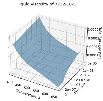
>>> water_mu.plot_TP_dependent_property(Tmin=400, Pmin=1e5, Pmax=1e8, methods_P=['COOLPROP','LUCAS'], pts=15, only_valid=False) 

(Source code, png, hires.png, pdf)

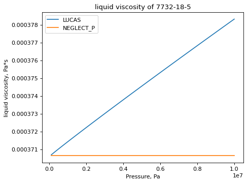
This can be a little confusing; but isotherms and isobars can be plotted as well, which are more straight forward. The respective methods are plot_isotherm and plot_isobar:

>>> water_mu.plot_isotherm(T=350, Pmin=1e5, Pmax=1e7, pts=50) 

(Source code, png, hires.png, pdf)

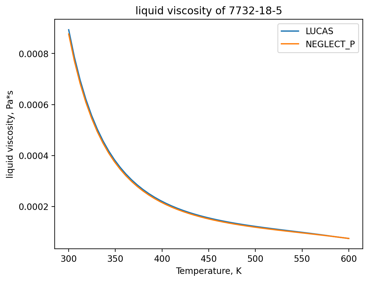
>>> water_mu.plot_isobar(P=1e7, Tmin=300, Tmax=600, pts=50) 

(Source code, png, hires.png, pdf)

Calculating Conditions From Properties

The method is solve_property works only on the low-pressure correlations.

>>> water_mu.solve_property(1e-3)  
294.0711641

Property Derivatives

Functionality for calculating the temperature derivative of the property is implemented twice; as T_dependent_property_derivative using the low-pressure correlations, and as TP_dependent_property_derivative_T using the high-pressure correlations that require pressure as an input.

>>> water_mu.T_dependent_property_derivative(300)  
-1.893961e-05
>>> water_mu.TP_dependent_property_derivative_T(300, P=1e7) 
-1.927268e-05

The derivatives are numerical unless a special implementation has been added to the property’s calculate_derivative_T and/or calculate_derivative method.

Higher order derivatives are available as well with the order argument.

>>> water_mu.T_dependent_property_derivative(300.0, order=2) 
5.923372e-07
>>> water_mu.TP_dependent_property_derivative_T(300.0, P=1e6, order=2) 
-1.40946e-06

Functionality for calculating the pressure derivative of the property is also implemented as TP_dependent_property_derivative_P:

>>> water_mu.TP_dependent_property_derivative_P(P=5e7, T=400) 
4.27782809e-13

The derivatives are numerical unless a special implementation has been added to the property’s calculate_derivative_P method.

Higher order derivatives are available as well with the order argument.

>>> water_mu.TP_dependent_property_derivative_P(P=5e7, T=400, order=2)  
-1.1858461e-15

Property Integrals

The same functionality for integrating over a property as in temperature-dependent objects is available, but only for integrating over temperature using low pressure correlations. No other use cases have been identified requiring integration over high-pressure conditions, or integration over the pressure domain.

>>> water_mu.T_dependent_property_integral(300, 400) # Integrating over viscosity has no physical meaning  
0.04243

Using Tabular Data

If there are experimentally available data for a property at high and low pressure, an interpolation table can be created and used as follows. The CoolProp method is used to generate a small table, and is then added as a new method in the example below.

>>> from thermo import *
>>> import numpy as np
>>> Ts = [300, 400, 500]
>>> Ps = [1e5, 1e6, 1e7]
>>> table = [[water_mu.calculate_P(T, P, "COOLPROP") for T in Ts] for P in Ps]  
>>> water_mu.method_P
'LUCAS'
>>> water_mu.add_tabular_data_P(Ts, Ps, table)  
>>> water_mu.method_P  
'Tabular data series #0'
>>> water_mu(400, 1e7), water_mu.calculate_P(400, 1e7, "COOLPROP")  
(0.000221166933349, 0.000221166933349)
>>> water_mu(450, 5e6), water_mu.calculate_P(450, 5e6, "COOLPROP")  
(0.00011340, 0.00015423)

The more data points used, the closer a property will match.

Mixture Properties

Notes

There is also the challenge that there is no clear criteria for distinguishing liquids from gases in supercritical mixtures. If the same method is not used for liquids and gases, there will be a sudden discontinuity which can cause numerical issues in modeling.